Mathematical fidelity: These page images preserve the exact notation and visual layout of the supplied PDF. The optional text extract below is for searching/copying only and may contain transcription errors.
Original pages — equations and symbols preserved
Show extracted text (searchable; equations may be imperfect)
Extract · PDF page 1
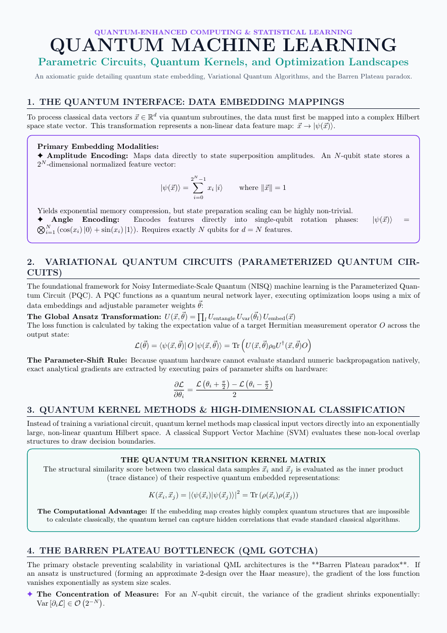
QUANTUM-ENHANCED COMPUTING & STATISTICAL LEARNING
QUANTUM MACHINE LEARNING
Parametric Circuits, Quantum Kernels, and Optimization Landscapes
An axiomatic guide detailing quantum state embedding, Variational Quantum Algorithms, and the Barren Plateau paradox.
Extract · PDF page 1
1. THE QUANTUM INTERFACE: DATA EMBEDDING MAPPINGS
To process classical data vectors ⃗x ∈Rd via quantum subroutines, the data must first be mapped into a complex Hilbert
space state vector. This transformation represents a non-linear data feature map: ⃗x →|ψ(⃗x)⟩.
Primary Embedding Modalities:
✦Amplitude Encoding: Maps data directly to state superposition amplitudes. An N-qubit state stores a
2N-dimensional normalized feature vector:
2N−1
|ψ(⃗x)⟩= X xi |i⟩ where ∥⃗x∥= 1
i=0
Yields exponential memory compression, but state preparation scaling can be highly non-trivial.
✦ Angle Encoding: Encodes features directly into single-qubit rotation phases: |ψ(⃗x)⟩ =
NNi=1 (cos(xi) |0⟩+ sin(xi) |1⟩). Requires exactly N qubits for d = N features.
Extract · PDF page 1
2. VARIATIONAL QUANTUM CIRCUITS (PARAMETERIZED QUANTUM CIR-
CUITS)
The foundational framework for Noisy Intermediate-Scale Quantum (NISQ) machine learning is the Parameterized Quan-
tum Circuit (PQC). A PQC functions as a quantum neural network layer, executing optimization loops using a mix of
data embeddings and adjustable parameter weights ⃗θ:
The Global Ansatz Transformation: U(⃗x, ⃗θ) = Ql Uentangle Uvar(⃗θl) Uembed(⃗x)
The loss function is calculated by taking the expectation value of a target Hermitian measurement operator O across the
output state:
L(⃗θ) = ⟨ψ(⃗x, ⃗θ)| O |ψ(⃗x, ⃗θ)⟩= Tr U(⃗x, ⃗θ)ρ0U †(⃗x, ⃗θ)O
The Parameter-Shift Rule: Because quantum hardware cannot evaluate standard numeric backpropagation natively,
exact analytical gradients are extracted by executing pairs of parameter shifts on hardware:
∂L L θi + π2 −L θi −π2 =
∂θi 2
Extract · PDF page 1
3. QUANTUM KERNEL METHODS & HIGH-DIMENSIONAL CLASSIFICATION
Instead of training a variational circuit, quantum kernel methods map classical input vectors directly into an exponentially
large, non-linear quantum Hilbert space. A classical Support Vector Machine (SVM) evaluates these non-local overlap
structures to draw decision boundaries.
THE QUANTUM TRANSITION KERNEL MATRIX
The structural similarity score between two classical data samples ⃗xi and ⃗xj is evaluated as the inner product
(trace distance) of their respective quantum embedded representations:
K(⃗xi, ⃗xj) = |⟨ψ(⃗xi)|ψ(⃗xj)⟩|2 = Tr (ρ(⃗xi)ρ(⃗xj))
The Computational Advantage: If the embedding map creates highly complex quantum structures that are impossible
to calculate classically, the quantum kernel can capture hidden correlations that evade standard classical algorithms.
Extract · PDF page 1
4. THE BARREN PLATEAU BOTTLENECK (QML GOTCHA)
The primary obstacle preventing scalability in variational QML architectures is the **Barren Plateau paradox**. If
an ansatz is unstructured (forming an approximate 2-design over the Haar measure), the gradient of the loss function
vanishes exponentially as system size scales.
✦The Concentration of Measure: For an N-qubit circuit, the variance of the gradient shrinks exponentially:
Var [∂iL] ∈O 2−N .
Extract · PDF page 2
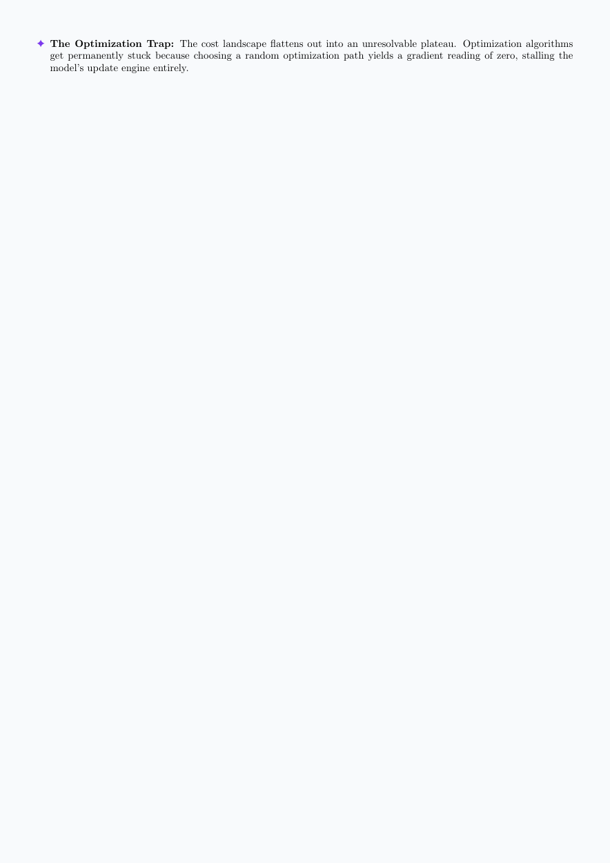
✦The Optimization Trap: The cost landscape flattens out into an unresolvable plateau. Optimization algorithms
get permanently stuck because choosing a random optimization path yields a gradient reading of zero, stalling the
model’s update engine entirely.