ℏThe Schrodinger Equation

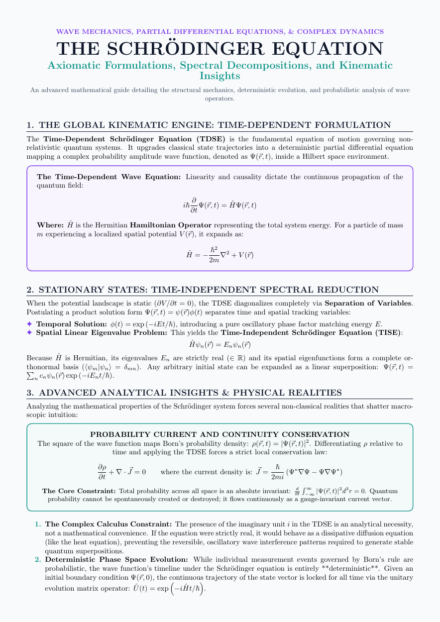
WAVE MECHANICS, PARTIAL DIFFERENTIAL EQUATIONS, & COMPLEX DYNAMICS THE SCHR¨ODINGER EQUATION Axiomatic Formulations, Spectral Decompositions, and Kinematic Insights An advanced mathematical guide detailing the structural mechanics, deterministic evolution, and probabilistic analysis of wave operators.

1. THE GLOBAL KINEMATIC ENGINE: TIME-DEPENDENT FORMULATION The Time-Dependent Schr¨odinger Equation (TDSE) is the fundamental equation of motion governing non- relativistic quantum systems. It upgrades classical state trajectories into a deterministic partial differential equation mapping a complex probability amplitude wave function, denoted as Ψ(⃗r, t), inside a Hilbert space environment. The Time-Dependent Wave Equation: Linearity and causality dictate the continuous propagation of the quantum field: iℏ∂ t) = ˆHΨ(⃗r, t) ∂tΨ(⃗r, Where: ˆH is the Hermitian Hamiltonian Operator representing the total system energy. For a particle of mass m experiencing a localized spatial potential V (⃗r), it expands as: ˆH = −ℏ2 + V (⃗r) 2m∇2

2. STATIONARY STATES: TIME-INDEPENDENT SPECTRAL REDUCTION When the potential landscape is static (∂V/∂t = 0), the TDSE diagonalizes completely via Separation of Variables. Postulating a product solution form Ψ(⃗r, t) = ψ(⃗r)ϕ(t) separates time and spatial tracking variables: ✦Temporal Solution: ϕ(t) = exp (−iEt/ℏ), introducing a pure oscillatory phase factor matching energy E. ✦Spatial Linear Eigenvalue Problem: This yields the Time-Independent Schr¨odinger Equation (TISE): ˆHψn(⃗r) = Enψn(⃗r) Because ˆH is Hermitian, its eigenvalues En are strictly real (∈R) and its spatial eigenfunctions form a complete or- thonormal basis (⟨ψm|ψn⟩= δmn). Any arbitrary initial state can be expanded as a linear superposition: Ψ(⃗r, t) = Pn cnψn(⃗r) exp (−iEnt/ℏ).

3. ADVANCED ANALYTICAL INSIGHTS & PHYSICAL REALITIES Analyzing the mathematical properties of the Schr¨odinger system forces several non-classical realities that shatter macro- scopic intuition: PROBABILITY CURRENT AND CONTINUITY CONSERVATION The square of the wave function maps Born’s probability density: ρ(⃗r, t) = |Ψ(⃗r, t)|2. Differentiating ρ relative to time and applying the TDSE forces a strict local conservation law: ∂ρ ℏ + ∇· ⃗J = 0 where the current density is: ⃗J = (Ψ∗∇Ψ −Ψ∇Ψ∗) ∂t 2mi The Core Constraint: Total probability across all space is an absolute invariant: dtd R −∞|Ψ(⃗r,∞ t)|2d3r = 0. Quantum probability cannot be spontaneously created or destroyed; it flows continuously as a gauge-invariant current vector. 1. The Complex Calculus Constraint: The presence of the imaginary unit i in the TDSE is an analytical necessity, not a mathematical convenience. If the equation were strictly real, it would behave as a dissipative diffusion equation (like the heat equation), preventing the reversible, oscillatory wave interference patterns required to generate stable quantum superpositions.

2. Deterministic Phase Space Evolution: While individual measurement events governed by Born’s rule are probabilistic, the wave function’s timeline under the Schr¨odinger equation is entirely **deterministic**. Given an initial boundary condition Ψ(⃗r, 0), the continuous trajectory of the state vector is locked for all time via the unitary evolution matrix operator: ˆU(t) = exp −iˆHt/ℏ .

∂2ψ 2m

3. Geometric Curvature & Kinetic Boundaries: Rewriting the TISE as ∂x2 = ℏ2 (V (x) −E)ψ maps energy to geometric curvature. Where E > V (x), the wave function curves toward the axis, yielding oscillatory profiles. Where E < V (x), the curvature flips away from the axis, forcing exponential decay. This smooth exponential boundary matching is the explicit engine behind **Quantum Tunneling**.