ℏClassical Precursors To Quantum

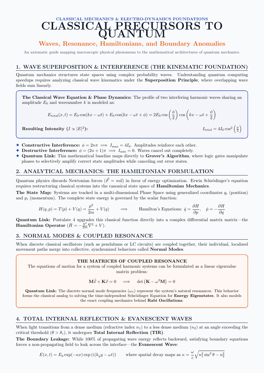
CLASSICAL MECHANICS & ELECTRO-DYNAMICS FOUNDATIONS CLASSICAL PRECURSORS TO QUANTUM Waves, Resonance, Hamiltonians, and Boundary Anomalies An axiomatic guide mapping macroscopic physical phenomena to the mathematical architectures of quantum mechanics.

1. WAVE SUPERPOSITION & INTERFERENCE (THE KINEMATIC FOUNDATION) Quantum mechanics structures state spaces using complex probability waves. Understanding quantum computing speedups requires analyzing classical wave kinematics under the Superposition Principle, where overlapping wave fields sum linearly. The Classical Wave Equation & Phase Dynamics: The profile of two interfering harmonic waves sharing an amplitude E0 and wavenumber k is modeled as: ϕ ϕ Etotal(x, t) = E0 cos(kx −ωt) + E0 cos(kx −ωt + ϕ) = 2E0 cos cos kx −ωt + 2 2 Resulting Intensity (I ∝|E|2): Itotal = 4I0 cos2 ϕ2 ✦Constructive Interference: ϕ = 2nπ =⇒Imax = 4I0. Amplitudes reinforce each other. ✦Destructive Interference: ϕ = (2n + 1)π =⇒Imin = 0. Waves cancel out completely. ✦Quantum Link: This mathematical baseline maps directly to Grover’s Algorithm, where logic gates manipulate phases to selectively amplify correct state amplitudes while canceling out error states.

2. ANALYTICAL MECHANICS: THE HAMILTONIAN FORMULATION Quantum physics discards Newtonian forces (⃗F = m⃗a) in favor of energy optimization. Erwin Schr¨odinger’s equation requires restructuring classical systems into the canonical state space of Hamiltonian Mechanics. The State Map: Systems are tracked in a multi-dimensional Phase Space using generalized coordinates qi (position) and pi (momentum). The complete state energy is governed by the scalar function: p2 ∂H H(q, p) = T(p) + V (q) = + V (q) =⇒ Hamilton’s Equations: ˙q = , ˙p = −∂H 2m ∂p ∂q Quantum Link: Postulate 4 upgrades this classical function directly into a complex differential matrix matrix—the Hamiltonian Operator ( ˆH = −ℏ22m∇2 + V ).

3. NORMAL MODES & COUPLED RESONANCE When discrete classical oscillators (such as pendulums or LC circuits) are coupled together, their individual, localized movement paths merge into collective, synchronized behaviors called Normal Modes. THE MATRICES OF COUPLED RESONANCE The equations of motion for a system of coupled harmonic systems can be formulated as a linear eigenvalue matrix problem: M¨⃗x + K⃗x = 0 =⇒ det K −ω2M = 0 Quantum Link: The discrete normal mode frequencies (ωn) represent the system’s natural resonances. This behavior forms the classical analog to solving the time-independent Schr¨odinger Equation for Energy Eigenstates. It also models the exact coupling mechanics behind Rabi Oscillations.

4. TOTAL INTERNAL REFLECTION & EVANESCENT WAVES When light transitions from a dense medium (refractive index n1) to a less dense medium (n2) at an angle exceeding the critical threshold (θ > θc), it undergoes Total Internal Reflection (TIR). The Boundary Leakage: While 100% of propagating wave energy reflects backward, satisfying boundary equations forces a non-propagating field to leak across the interface—the Evanescent Wave: ω q E(x, t) = E0 exp(−κx) exp (i(kyy −ωt)) where spatial decay maps as κ = n21 sin2 θ −n22 c

Quantum Link: If a second dense medium is brought close to the boundary, light skips across the air gap. This classical phenomenon, called Frustrated Total Internal Reflection, utilizes the exact same exponential boundary equations that govern Quantum Tunneling and sub-wavelength field trapping in Nanophotonics.