ℏGreen'S Functions In Quantum

DIFFERENTIAL OPERATORS, MANY-BODY FIELD THEORY, & PROPAGATORS GREEN’S FUNCTIONS IN QUANTUM Impulse Responses, Time-Ordered Propagators, and Perturbation Theory An axiomatic mathematical guide detailing how Green’s functions solve interacting quantum differential equations.

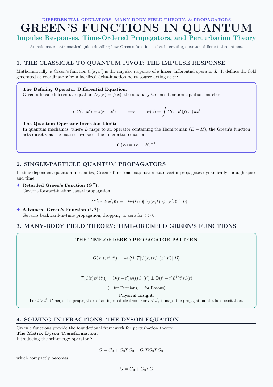
1. THE CLASSICAL TO QUANTUM PIVOT: THE IMPULSE RESPONSE Mathematically, a Green’s function G(x, x′) is the impulse response of a linear differential operator L. It defines the field generated at coordinate x by a localized delta-function point source acting at x′: The Defining Operator Differential Equation: Given a linear differential equation Lψ(x) = f(x), the auxiliary Green’s function equation matches: Z L G(x, x′) = δ(x −x′) =⇒ ψ(x) = G(x, x′)f(x′) dx′ The Quantum Operator Inversion Limit: In quantum mechanics, where L maps to an operator containing the Hamiltonian (E −H), the Green’s function acts directly as the matrix inverse of the differential equation: G(E) = (E −H)−1

2. SINGLE-PARTICLE QUANTUM PROPAGATORS In time-dependent quantum mechanics, Green’s functions map how a state vector propagates dynamically through space and time. ✦Retarded Green’s Function (GR): Governs forward-in-time causal propagation: GR(x, t; x′, 0) = −iΘ(t) ⟨0| {ψ(x, t), ψ†(x′, 0)} |0⟩ ✦Advanced Green’s Function (GA): Governs backward-in-time propagation, dropping to zero for t > 0.

3. MANY-BODY FIELD THEORY: TIME-ORDERED GREEN’S FUNCTIONS THE TIME-ORDERED PROPAGATOR PATTERN G(x, t; x′, t′) = −i ⟨Ω| T [ψ(x, t)ψ†(x′, t′)] |Ω⟩ T [ψ(t)ψ†(t′)] = Θ(t −t′)ψ(t)ψ†(t′) ± Θ(t′ −t)ψ†(t′)ψ(t) (−for Fermions, + for Bosons) Physical Insight: For t > t′, G maps the propagation of an injected electron. For t < t′, it maps the propagation of a hole excitation.

4. SOLVING INTERACTIONS: THE DYSON EQUATION Green’s functions provide the foundational framework for perturbation theory. The Matrix Dyson Transformation: Introducing the self-energy operator Σ: G = G0 + G0ΣG0 + G0ΣG0ΣG0 + . . . which compactly becomes G = G0 + G0ΣG

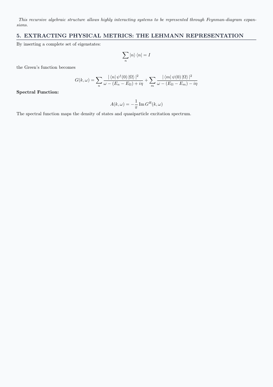
This recursive algebraic structure allows highly interacting systems to be represented through Feynman-diagram expan- sions.

5. EXTRACTING PHYSICAL METRICS: THE LEHMANN REPRESENTATION By inserting a complete set of eigenstates: X |n⟩⟨n| = I n the Green’s function becomes | ⟨n| ψ†(0) |Ω⟩|2 | ⟨m| ψ(0) |Ω⟩|2 G(k, ω) = X + X ω −(En −EΩ) + iη ω −(EΩ−Em) −iη n m Spectral Function: A(k, ω) = −1 Im GR(k, ω) π The spectral function maps the density of states and quasiparticle excitation spectrum.