Mathematical fidelity: These page images preserve the exact notation and visual layout of the supplied PDF. The optional text extract below is for searching/copying only and may contain transcription errors.
Original pages — equations and symbols preserved
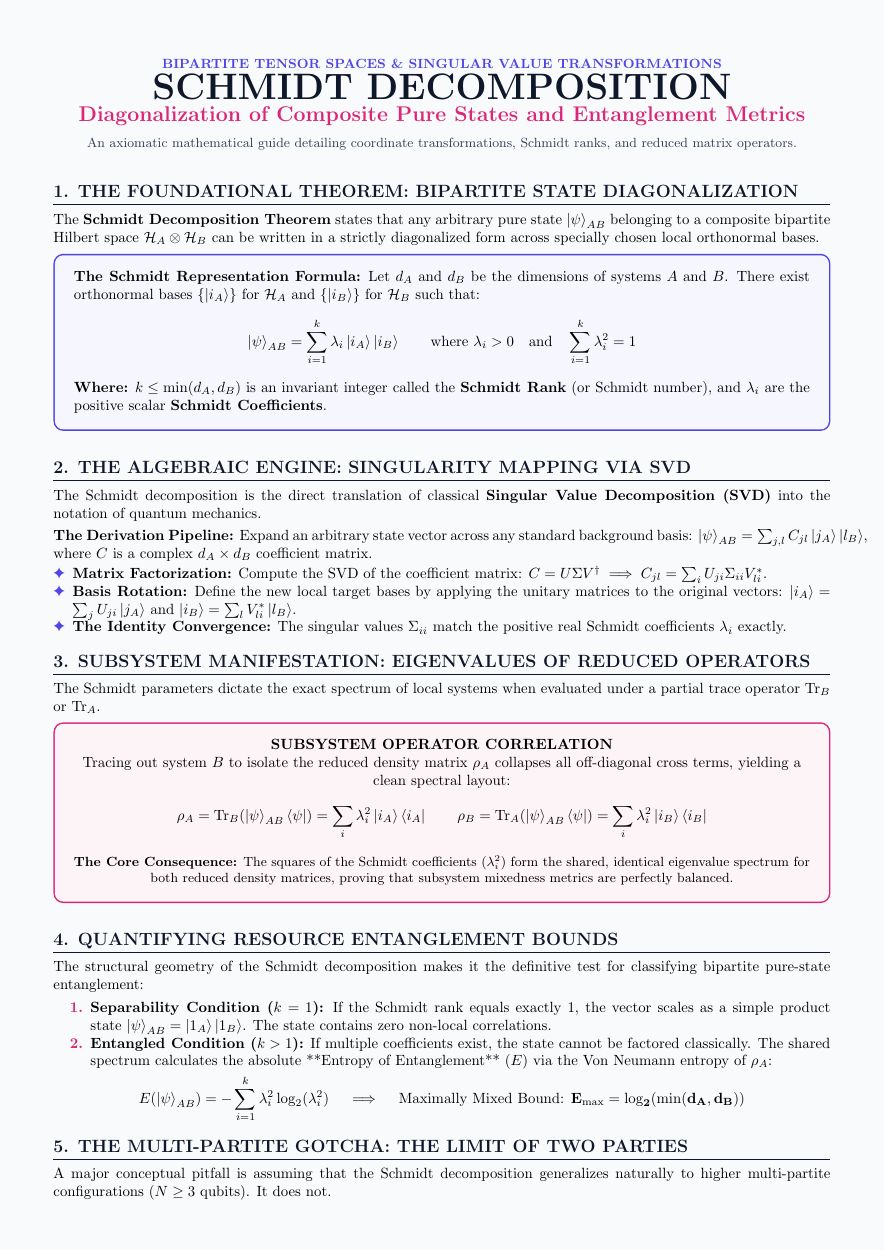

Show extracted text (searchable; equations may be imperfect)
Extract · PDF page 1
BIPARTITE TENSOR SPACES & SINGULAR VALUE TRANSFORMATIONS
SCHMIDT DECOMPOSITION
Diagonalization of Composite Pure States and Entanglement Metrics
An axiomatic mathematical guide detailing coordinate transformations, Schmidt ranks, and reduced matrix operators.
Extract · PDF page 1
1. THE FOUNDATIONAL THEOREM: BIPARTITE STATE DIAGONALIZATION
The Schmidt Decomposition Theorem states that any arbitrary pure state |ψ⟩AB belonging to a composite bipartite
Hilbert space HA ⊗HB can be written in a strictly diagonalized form across specially chosen local orthonormal bases.
The Schmidt Representation Formula: Let dA and dB be the dimensions of systems A and B. There exist
orthonormal bases {|iA⟩} for HA and {|iB⟩} for HB such that:
k k
|ψ⟩AB = X λi |iA⟩|iB⟩ where λi > 0 and X λ2i = 1
i=1 i=1
Where: k ≤min(dA, dB) is an invariant integer called the Schmidt Rank (or Schmidt number), and λi are the
positive scalar Schmidt Coefficients.
Extract · PDF page 1
2. THE ALGEBRAIC ENGINE: SINGULARITY MAPPING VIA SVD
The Schmidt decomposition is the direct translation of classical Singular Value Decomposition (SVD) into the
notation of quantum mechanics.
The Derivation Pipeline: Expand an arbitrary state vector across any standard background basis: |ψ⟩AB = Pj,l Cjl |jA⟩|lB⟩,
where C is a complex dA × dB coefficient matrix.
✦Matrix Factorization: Compute the SVD of the coefficient matrix: C = UΣV † =⇒Cjl = Pi UjiΣiiV li.∗
✦Basis Rotation: Define the new local target bases by applying the unitary matrices to the original vectors: |iA⟩=
Pj Uji |jA⟩and |iB⟩= Pl V li∗ |lB⟩.
✦The Identity Convergence: The singular values Σii match the positive real Schmidt coefficients λi exactly.
Extract · PDF page 1
3. SUBSYSTEM MANIFESTATION: EIGENVALUES OF REDUCED OPERATORS
The Schmidt parameters dictate the exact spectrum of local systems when evaluated under a partial trace operator TrB
or TrA.
SUBSYSTEM OPERATOR CORRELATION
Tracing out system B to isolate the reduced density matrix ρA collapses all off-diagonal cross terms, yielding a
clean spectral layout:
ρA = TrB(|ψ⟩AB ⟨ψ|) = X λ2i |iA⟩⟨iA| ρB = TrA(|ψ⟩AB ⟨ψ|) = X λ2i |iB⟩⟨iB|
i i
The Core Consequence: The squares of the Schmidt coefficients (λ2i ) form the shared, identical eigenvalue spectrum for
both reduced density matrices, proving that subsystem mixedness metrics are perfectly balanced.
Extract · PDF page 1
4. QUANTIFYING RESOURCE ENTANGLEMENT BOUNDS
The structural geometry of the Schmidt decomposition makes it the definitive test for classifying bipartite pure-state
entanglement:
1. Separability Condition (k = 1): If the Schmidt rank equals exactly 1, the vector scales as a simple product
state |ψ⟩AB = |1A⟩|1B⟩. The state contains zero non-local correlations.
2. Entangled Condition (k > 1): If multiple coefficients exist, the state cannot be factored classically. The shared
spectrum calculates the absolute **Entropy of Entanglement** (E) via the Von Neumann entropy of ρA:
k
E(|ψ⟩AB) = − X λ2i log2(λ2i ) =⇒ Maximally Mixed Bound: Emax = log2(min(dA, dB))
i=1
Extract · PDF page 1
5. THE MULTI-PARTITE GOTCHA: THE LIMIT OF TWO PARTIES
A major conceptual pitfall is assuming that the Schmidt decomposition generalizes naturally to higher multi-partite
configurations (N ≥3 qubits). It does not.
Extract · PDF page 2
|W⟩3 = √13(|100⟩+ |012⟩+ |001⟩) ←→ Cannot be diagonalized synchronously!
For three or more systems, it is mathematically impossible to construct localized transformations that simplify the global
state vector into a single index summation map Pi λi |iA⟩|iB⟩|iC⟩. Multi-partite spaces split into distinct SLOCC classes
(like GHZ vs. W), escaping single-diagonal matrix operations.