ℏThe Crámer-Rao Bound

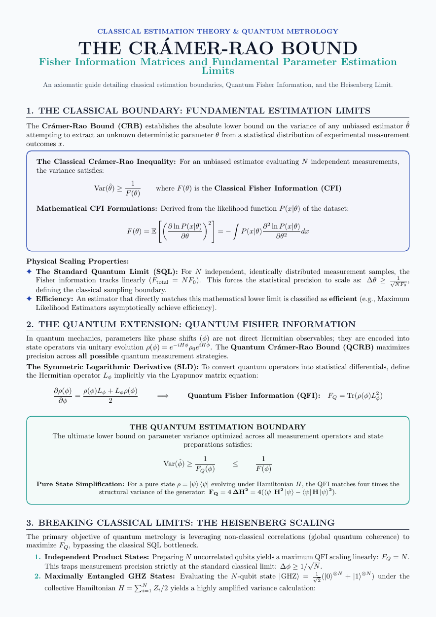
CLASSICAL ESTIMATION THEORY & QUANTUM METROLOGY THE CR´AMER-RAO BOUND Fisher Information Matrices and Fundamental Parameter Estimation Limits An axiomatic guide detailing classical estimation boundaries, Quantum Fisher Information, and the Heisenberg Limit.

1. THE CLASSICAL BOUNDARY: FUNDAMENTAL ESTIMATION LIMITS The Cr´amer-Rao Bound (CRB) establishes the absolute lower bound on the variance of any unbiased estimator ˆθ attempting to extract an unknown deterministic parameter θ from a statistical distribution of experimental measurement outcomes x. The Classical Cr´amer-Rao Inequality: For an unbiased estimator evaluating N independent measurements, the variance satisfies: 1 Var(ˆθ) ≥ where F(θ) is the Classical Fisher Information (CFI) F(θ) Mathematical CFI Formulations: Derived from the likelihood function P(x|θ) of the dataset: " 2# ∂ln P(x|θ) Z ln P(x|θ) F(θ) = E = − P(x|θ)∂2 dx ∂θ ∂θ2 Physical Scaling Properties: ✦The Standard Quantum Limit (SQL): For N independent, identically distributed measurement samples, the Fisher information tracks linearly (Ftotal = NF0). This forces the statistical precision to scale as: ∆θ ≥ √NF01 , defining the classical sampling boundary. ✦Efficiency: An estimator that directly matches this mathematical lower limit is classified as efficient (e.g., Maximum Likelihood Estimators asymptotically achieve efficiency).

2. THE QUANTUM EXTENSION: QUANTUM FISHER INFORMATION In quantum mechanics, parameters like phase shifts (ϕ) are not direct Hermitian observables; they are encoded into state operators via unitary evolution ρ(ϕ) = e−iHϕρ0eiHϕ. The Quantum Cr´amer-Rao Bound (QCRB) maximizes precision across all possible quantum measurement strategies. The Symmetric Logarithmic Derivative (SLD): To convert quantum operators into statistical differentials, define the Hermitian operator Lϕ implicitly via the Lyapunov matrix equation: ∂ρ(ϕ) ρ(ϕ)Lϕ + Lϕρ(ϕ) = =⇒ Quantum Fisher Information (QFI): FQ = Tr(ρ(ϕ)L2ϕ) ∂ϕ 2 THE QUANTUM ESTIMATION BOUNDARY The ultimate lower bound on parameter variance optimized across all measurement operators and state preparations satisfies: 1 1 Var(ˆϕ) ≥ ≤ FQ(ϕ) F(ϕ) Pure State Simplification: For a pure state ρ = |ψ⟩⟨ψ| evolving under Hamiltonian H, the QFI matches four times the structural variance of the generator: FQ = 4 ∆H2 = 4(⟨ψ| H2 |ψ⟩−⟨ψ| H |ψ⟩2).

3. BREAKING CLASSICAL LIMITS: THE HEISENBERG SCALING The primary objective of quantum metrology is leveraging non-classical correlations (global quantum coherence) to maximize FQ, bypassing the classical SQL bottleneck. 1. Independent Product States: Preparing N uncorrelated qubits yields a maximum QFI scaling linearly: FQ = N. √ This traps measurement precision strictly at the standard classical limit: ∆ϕ ≥1/ N.

2. Maximally Entangled GHZ States: Evaluating the N-qubit state |GHZ⟩= √12(|0⟩⊗N + |1⟩⊗N) under the collective Hamiltonian H = PNi=1 Zi/2 yields a highly amplified variance calculation:

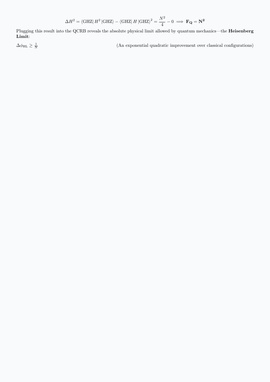
N 2 ∆H2 = ⟨GHZ| H2 |GHZ⟩−⟨GHZ| H |GHZ⟩2 = −0 =⇒FQ = N2 4 Plugging this result into the QCRB reveals the absolute physical limit allowed by quantum mechanics—the Heisenberg Limit: ∆ϕHL ≥1N (An exponential quadratic improvement over classical configurations)