Math fidelity: The original PDF page is displayed as a high-resolution image so that equations, bra–ket notation, matrix layouts and circuit diagrams remain exactly as in the source. The expandable text layer is for searching and may not reproduce every mathematical glyph.
Source page 1
Direct link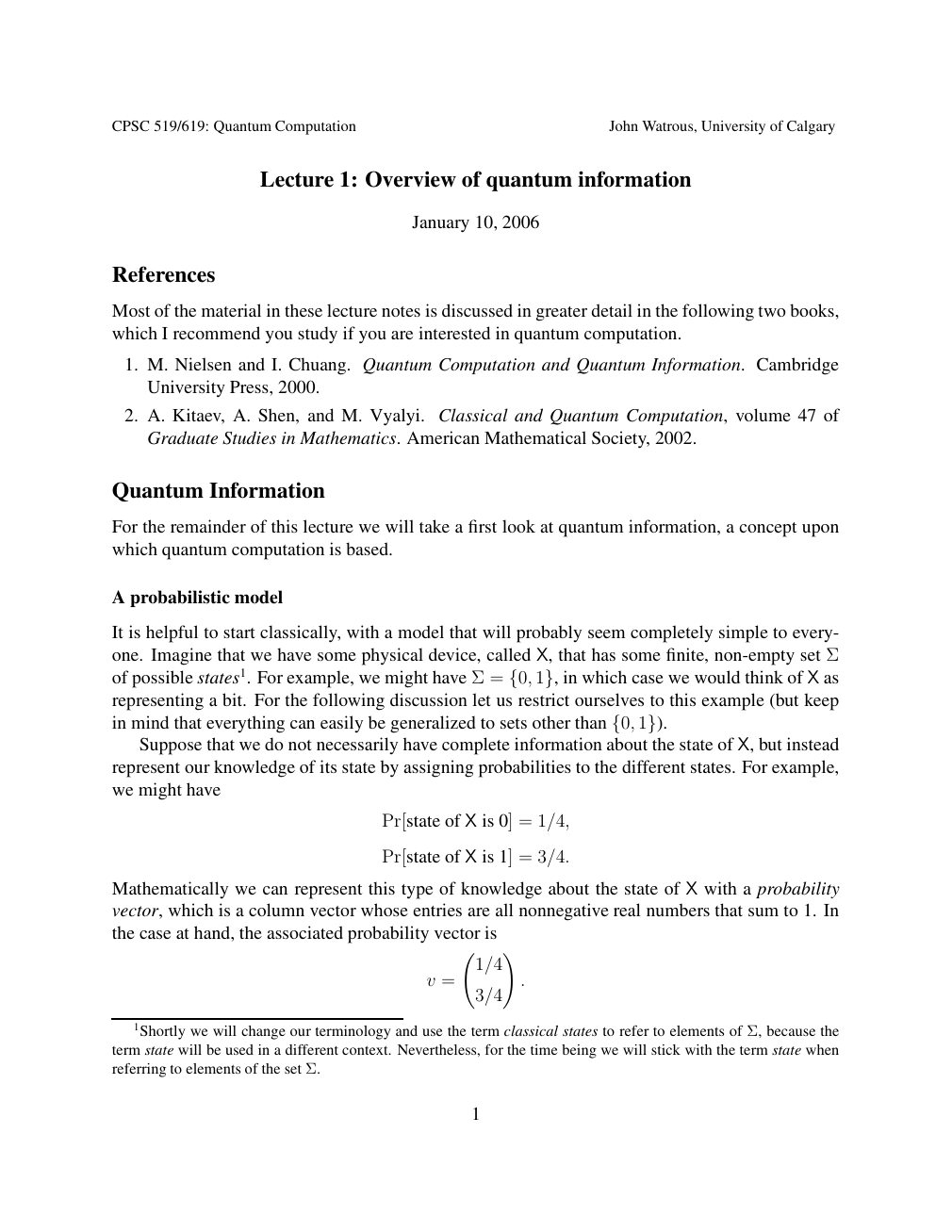
Show extracted searchable text (mathematical glyphs may differ)
CPSC 519/619: Quantum Computation John Watrous, University of Calgary
Lecture 1: Overview of quantum information
January 10, 2006
References
Most of the material in these lecture notes is discussed in greater detail in the following two books,
which I recommend you study if you are interested in quantum computation.
1. M. Nielsen and I. Chuang. Quantum Computation and Quantum Information. Cambridge
University Press, 2000.
2. A. Kitaev, A. Shen, and M. Vyalyi. Classical and Quantum Computation, volume 47 of
Graduate Studies in Mathematics. American Mathematical Society, 2002.
Quantum Information
For the remainder of this lecture we will take a first look at quantum information, a concept upon
which quantum computation is based.
A probabilistic model
It is helpful to start classically, with a model that will probably seem completely simple to every-
one. Imagine that we have some physical device, called X, that has some finite, non-empty set Σ
of possible states1. For example, we might have Σ = in which case we would think of X as {0, 1},representing a bit. For the following discussion let us restrict ourselves to this example (but keep
in mind that everything can easily be generalized to sets other than {0, 1}). Suppose that we do not necessarily have complete information about the state of X, but instead
represent our knowledge of its state by assigning probabilities to the different states. For example,
we might have
Pr[state of X is 0] = 1/4,
Pr[state of X is 1] = 3/4.
Mathematically we can represent this type of knowledge about the state of X with a probability
vector, which is a column vector whose entries are all nonnegative real numbers that sum to 1. In
the case at hand, the associated probability vector is
!
1/4
v = .
3/4
1Shortly we will change our terminology and use the term classical states to refer to elements of Σ, because the
term state will be used in a different context. Nevertheless, for the time being we will stick with the term state when
referring to elements of the set Σ.
1
Source page 2
Direct link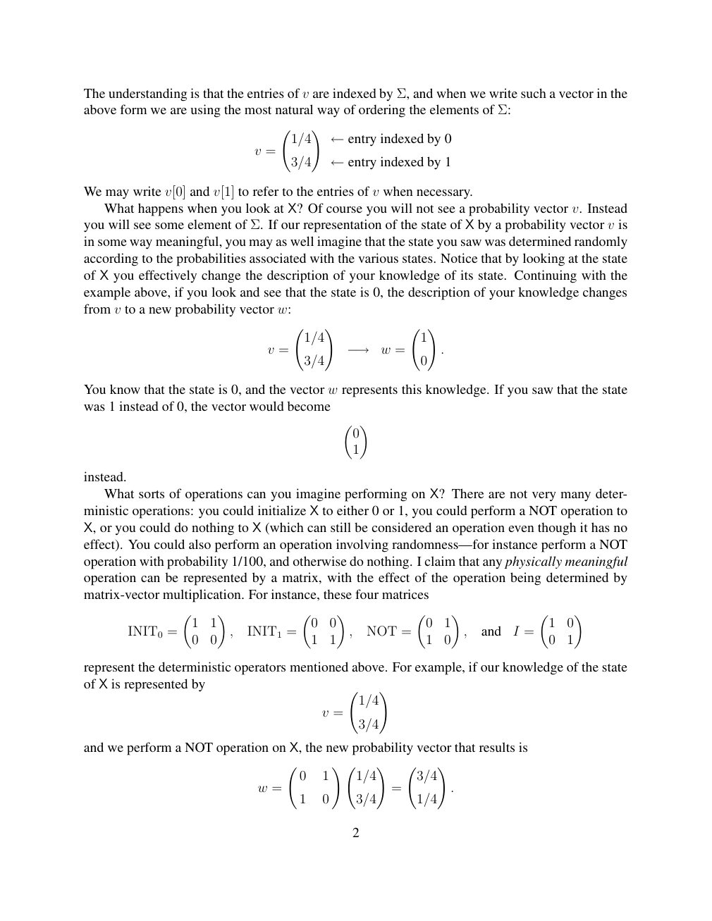
Show extracted searchable text (mathematical glyphs may differ)
The understanding is that the entries of v are indexed by Σ, and when we write such a vector in the
above form we are using the most natural way of ordering the elements of Σ:
!
1/4 ←entry indexed by 0 v =
3/4 ←entry indexed by 1
We may write v[0] and v[1] to refer to the entries of v when necessary.
What happens when you look at X? Of course you will not see a probability vector v. Instead
you will see some element of Σ. If our representation of the state of X by a probability vector v is
in some way meaningful, you may as well imagine that the state you saw was determined randomly
according to the probabilities associated with the various states. Notice that by looking at the state
of X you effectively change the description of your knowledge of its state. Continuing with the
example above, if you look and see that the state is 0, the description of your knowledge changes
from v to a new probability vector w:
! !
1/4 1
v = 3/4 −→ w = 0 .
You know that the state is 0, and the vector w represents this knowledge. If you saw that the state
was 1 instead of 0, the vector would become
0
1
instead.
What sorts of operations can you imagine performing on X? There are not very many deter-
ministic operations: you could initialize X to either 0 or 1, you could perform a NOT operation to
X, or you could do nothing to X (which can still be considered an operation even though it has no
effect). You could also perform an operation involving randomness—for instance perform a NOT
operation with probability 1/100, and otherwise do nothing. I claim that any physically meaningful
operation can be represented by a matrix, with the effect of the operation being determined by
matrix-vector multiplication. For instance, these four matrices
1 1 0 0 0 1 1 0 INIT0 = , INIT1 = , NOT = , and I =
0 0 1 1 1 0 0 1
represent the deterministic operators mentioned above. For example, if our knowledge of the state
of X is represented by !
1/4
v =
3/4
and we perform a NOT operation on X, the new probability vector that results is
! ! !
0 1 1/4 3/4
w = = .
1 0 3/4 1/4
2
Source page 3
Direct link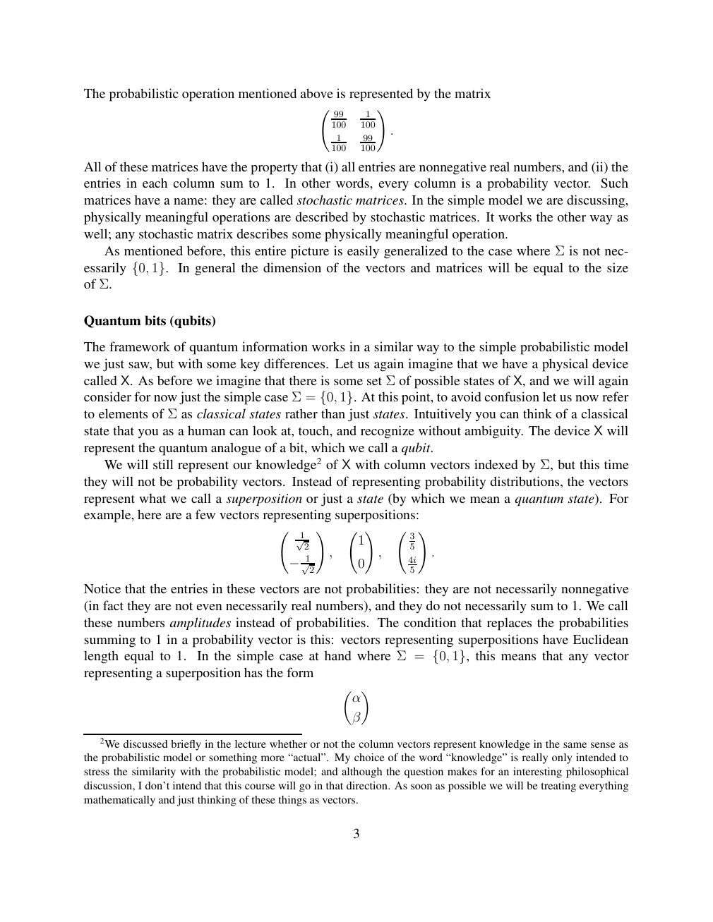
Show extracted searchable text (mathematical glyphs may differ)
The probabilistic operation mentioned above is represented by the matrix
!
99 1
100 100
.
1 99
100 100
All of these matrices have the property that (i) all entries are nonnegative real numbers, and (ii) the
entries in each column sum to 1. In other words, every column is a probability vector. Such
matrices have a name: they are called stochastic matrices. In the simple model we are discussing,
physically meaningful operations are described by stochastic matrices. It works the other way as
well; any stochastic matrix describes some physically meaningful operation.
As mentioned before, this entire picture is easily generalized to the case where Σ is not nec-
essarily In general the dimension of the vectors and matrices will be equal to the size {0, 1}.of Σ.
Quantum bits (qubits)
The framework of quantum information works in a similar way to the simple probabilistic model
we just saw, but with some key differences. Let us again imagine that we have a physical device
called X. As before we imagine that there is some set Σ of possible states of X, and we will again
consider for now just the simple case Σ = At this point, to avoid confusion let us now refer {0, 1}.to elements of Σ as classical states rather than just states. Intuitively you can think of a classical
state that you as a human can look at, touch, and recognize without ambiguity. The device X will
represent the quantum analogue of a bit, which we call a qubit.
We will still represent our knowledge2 of X with column vectors indexed by Σ, but this time
they will not be probability vectors. Instead of representing probability distributions, the vectors
represent what we call a superposition or just a state (by which we mean a quantum state). For
example, here are a few vectors representing superpositions:
! ! !
1 1 3 √ 2 5
, , .
√ 2 0 4i5 −1
Notice that the entries in these vectors are not probabilities: they are not necessarily nonnegative
(in fact they are not even necessarily real numbers), and they do not necessarily sum to 1. We call
these numbers amplitudes instead of probabilities. The condition that replaces the probabilities
summing to 1 in a probability vector is this: vectors representing superpositions have Euclidean
length equal to 1. In the simple case at hand where Σ = this means that any vector {0, 1},representing a superposition has the form
α
β
2We discussed briefly in the lecture whether or not the column vectors represent knowledge in the same sense as
the probabilistic model or something more “actual”. My choice of the word “knowledge” is really only intended to
stress the similarity with the probabilistic model; and although the question makes for an interesting philosophical
discussion, I don’t intend that this course will go in that direction. As soon as possible we will be treating everything
mathematically and just thinking of these things as vectors.
3
Source page 4
Direct link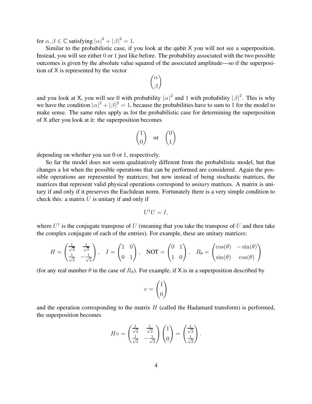
Show extracted searchable text (mathematical glyphs may differ)
for α, β satisfying + = 1. ∈C |α|2 |β|2 X Similar to the probabilistic case, if you look at the qubit you will not see a superposition.
Instead, you will see either 0 or 1 just like before. The probability associated with the two possible
outcomes is given by the absolute value squared of the associated amplitude—so if the superposi-
tion of X is represented by the vector
α
β
and you look at X, you will see 0 with probability |α|2 and 1 with probability |β|2. This is why
we have the condition |α|2 + |β|2 = 1, because the probabilities have to sum to 1 for the model tomake sense. The same rules apply as for the probabilistic case for determining the superposition
of X after you look at it: the superposition becomes
1 0
or
0 1
depending on whether you see 0 or 1, respectively.
So far the model does not seem qualitatively different from the probabilistic model, but that
changes a lot when the possible operations that can be performed are considered. Again the pos-
sible operations are represented by matrices; but now instead of being stochastic matrices, the
matrices that represent valid physical operations correspond to unitary matrices. A matrix is uni-
tary if and only if it preserves the Euclidean norm. Fortunately there is a very simple condition to
check this: a matrix U is unitary if and only if
U †U = I,
where U † is the conjugate transpose of U (meaning that you take the transpose of U and then take
the complex conjugate of each of the entries). For example, these are unitary matrices:
! ! ! !
1 1
1 0 0 1 √ 2 √ 2 cos(θ) −sin(θ) , I = H = , NOT = , Rθ = 1
√2 √ 2 0 1 1 0 sin(θ) cos(θ) −1
(for any real number θ in the case of Rθ). For example, if X is in a superposition described by
!
1
v =
0
and the operation corresponding to the matrix H (called the Hadamard transform) is performed,
the superposition becomes
! ! !
1 1
√ 2 √ 2 1 √12
Hv = = . 1
√ 2 √2 0 √12 −1
4
Source page 5
Direct link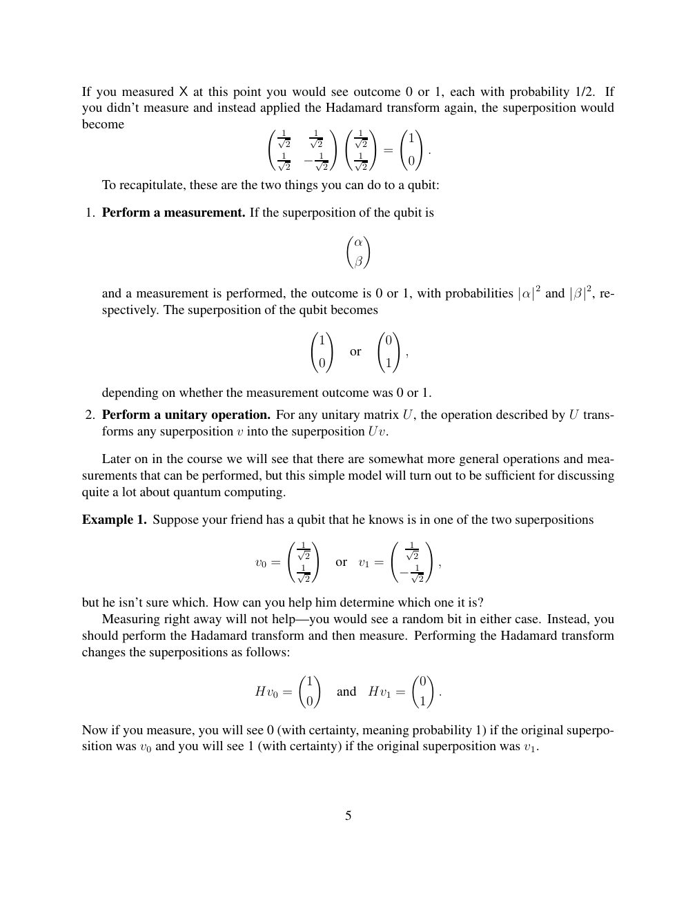
Show extracted searchable text (mathematical glyphs may differ)
If you measured X at this point you would see outcome 0 or 1, each with probability 1/2. If
you didn’t measure and instead applied the Hadamard transform again, the superposition would
become ! ! !
1 1 1
1 √ 2 √ 2 √ 2
= . 1 1
0 √ 2 √2 √ 2 −1
To recapitulate, these are the two things you can do to a qubit:
1. Perform a measurement. If the superposition of the qubit is
α
β
and a measurement is performed, the outcome is 0 or 1, with probabilities |α|2 and |β|2, re- spectively. The superposition of the qubit becomes
! !
1 0
or ,
0 1
depending on whether the measurement outcome was 0 or 1.
2. Perform a unitary operation. For any unitary matrix U, the operation described by U trans-
forms any superposition v into the superposition Uv.
Later on in the course we will see that there are somewhat more general operations and mea-
surements that can be performed, but this simple model will turn out to be sufficient for discussing
quite a lot about quantum computing.
Example 1. Suppose your friend has a qubit that he knows is in one of the two superpositions
! !
1 1
√2 √2 or v1 = , v0 = 1
√2 √2 −1
but he isn’t sure which. How can you help him determine which one it is?
Measuring right away will not help—you would see a random bit in either case. Instead, you
should perform the Hadamard transform and then measure. Performing the Hadamard transform
changes the superpositions as follows:
1 0
Hv0 = and Hv1 = .
0 1
Now if you measure, you will see 0 (with certainty, meaning probability 1) if the original superpo-
sition was v0 and you will see 1 (with certainty) if the original superposition was v1.
5
⊗ Circuit walkthrough: entanglement and measurement
The Hadamard gate prepares (|0⟩ + |1⟩)/√2 on the first qubit. The controlled-NOT then creates the Bell state (|00⟩ + |11⟩)/√2. Measuring both qubits in the computational basis produces correlated 00 and 11 outcomes, each with ideal probability 1/2. This example illustrates a circuit building block; it is not a complete implementation of the surrounding algorithm.
Show runnable Qiskit example
from qiskit import QuantumCircuit
from qiskit_aer import AerSimulator

qc = QuantumCircuit(2, 2)
qc.h(0)             # Superpose the first qubit
qc.cx(0, 1)         # Entangle both qubits
qc.measure([0, 1], [0, 1])
print(qc.draw(output="text"))
result = AerSimulator().run(qc, shots=1024).result()
print(result.get_counts())  # Approximately 00 and 11
Install qiskit and qiskit-aer locally to execute this code. The diagram is a static circuit illustration, not a browser-based simulator.