Math fidelity: The original PDF page is displayed as a high-resolution image so that equations, bra–ket notation, matrix layouts and circuit diagrams remain exactly as in the source. The expandable text layer is for searching and may not reproduce every mathematical glyph.
Source page 28
Direct link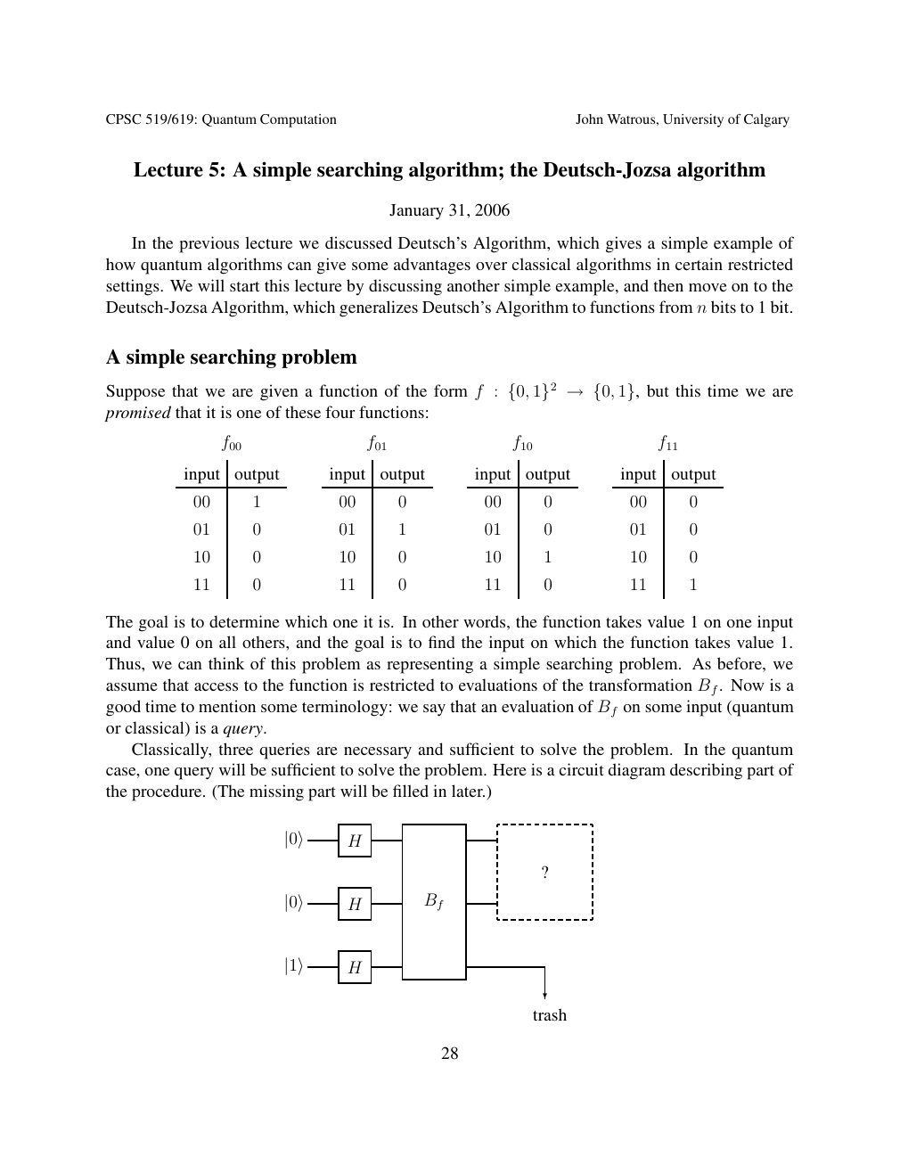
Show extracted searchable text (mathematical glyphs may differ)
CPSC 519/619: Quantum Computation John Watrous, University of Calgary
Lecture 5: A simple searching algorithm; the Deutsch-Jozsa algorithm
January 31, 2006
In the previous lecture we discussed Deutsch’s Algorithm, which gives a simple example of
how quantum algorithms can give some advantages over classical algorithms in certain restricted
settings. We will start this lecture by discussing another simple example, and then move on to the
Deutsch-Jozsa Algorithm, which generalizes Deutsch’s Algorithm to functions from n bits to 1 bit.
A simple searching problem
Suppose that we are given a function of the form f : but this time we are {0, 1}2 →{0, 1},promised that it is one of these four functions:
f00 f01 f10 f11
input output input output input output input output
00 1 00 0 00 0 00 0
01 0 01 1 01 0 01 0
10 0 10 0 10 1 10 0
11 0 11 0 11 0 11 1
The goal is to determine which one it is. In other words, the function takes value 1 on one input
and value 0 on all others, and the goal is to find the input on which the function takes value 1.
Thus, we can think of this problem as representing a simple searching problem. As before, we
assume that access to the function is restricted to evaluations of the transformation Bf. Now is a
good time to mention some terminology: we say that an evaluation of Bf on some input (quantum
or classical) is a query.
Classically, three queries are necessary and sufficient to solve the problem. In the quantum
case, one query will be sufficient to solve the problem. Here is a circuit diagram describing part of
the procedure. (The missing part will be filled in later.)
|0⟩ H
?
|0⟩ H Bf
|1⟩ H
?
trash
28
Source page 29
Direct link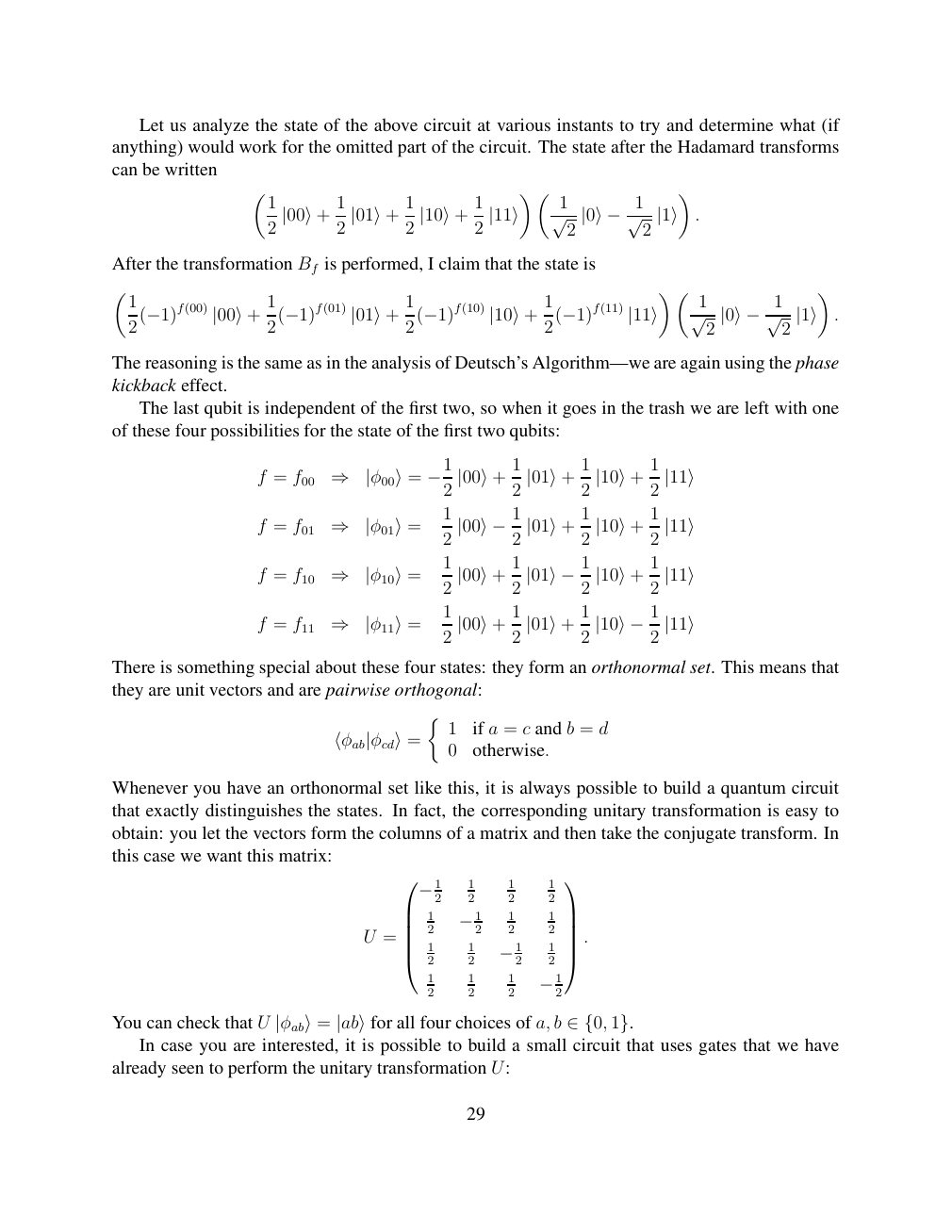
Show extracted searchable text (mathematical glyphs may differ)
Let us analyze the state of the above circuit at various instants to try and determine what (if
anything) would work for the omitted part of the circuit. The state after the Hadamard transforms
can be written
1 1 1 1 1
. 2 |00⟩+ 2 |01⟩+ 2 |10⟩+ 2 |11⟩ √ 2 |0⟩−1√ 2 |1⟩
After the transformation Bf is performed, I claim that the state is
1 1 1 1 1
. 2(−1)f(00) |00⟩+ 2(−1)f(01) |01⟩+ 2(−1)f(10) |10⟩+ 2(−1)f(11) |11⟩ √ 2 |0⟩−1√ 2 |1⟩
The reasoning is the same as in the analysis of Deutsch’s Algorithm—we are again using the phase
kickback effect.
The last qubit is independent of the first two, so when it goes in the trash we are left with one
of these four possibilities for the state of the first two qubits:
1 1 1
f = f00 ⇒ |φ00⟩= −12 |00⟩+ 2 |01⟩+ 2 |10⟩+ 2 |11⟩
1 1 1
f = f01 ⇒ |φ01⟩= 2 |00⟩−12 |01⟩+ 2 |10⟩+ 2 |11⟩
1 1 1
f = f10 ⇒ |φ10⟩= 2 |00⟩+ 2 |01⟩−12 |10⟩+ 2 |11⟩
1 1 1
f = f11 ⇒ |φ11⟩= 2 |00⟩+ 2 |01⟩+ 2 |10⟩−12 |11⟩
There is something special about these four states: they form an orthonormal set. This means that
they are unit vectors and are pairwise orthogonal:
1 if a = c and b = d
⟨φab|φcd⟩= 0 otherwise.
Whenever you have an orthonormal set like this, it is always possible to build a quantum circuit
that exactly distinguishes the states. In fact, the corresponding unitary transformation is easy to
obtain: you let the vectors form the columns of a matrix and then take the conjugate transform. In
this case we want this matrix:
1 1 1
2 2 2 2 −1 1 1 1
2 2 2 2 −1 . U = 1 1 1
2 2 2 2 −1
1 1 1
2 2 2 2 −1
You can check that U all four choices of a, b |φab⟩= |ab⟩for ∈{0, 1}. In case you are interested, it is possible to build a small circuit that uses gates that we have
already seen to perform the unitary transformation U:
29
Source page 30
Direct link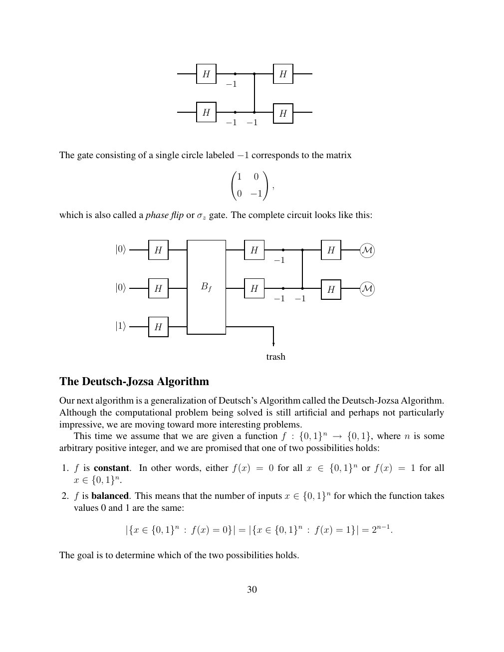
Show extracted searchable text (mathematical glyphs may differ)
H H
−1
H H
−1 −1
The gate consisting of a single circle labeled corresponds to the matrix −1
!
1 0
,
0 −1
which is also called a phase flip or σz gate. The complete circuit looks like this:
|0⟩ H H H M
−1
|0⟩ H Bf H H M
−1 −1
|1⟩ H
?
trash
The Deutsch-Jozsa Algorithm
Our next algorithm is a generalization of Deutsch’s Algorithm called the Deutsch-Jozsa Algorithm.
Although the computational problem being solved is still artificial and perhaps not particularly
impressive, we are moving toward more interesting problems.
This time we assume that we are given a function f : where n is some {0, 1}n →{0, 1},arbitrary positive integer, and we are promised that one of two possibilities holds:
1. f is constant. In other words, either f(x) = 0 for all x or f(x) = 1 for all ∈{0, 1}n
x ∈{0, 1}n.
2. f is balanced. This means that the number of inputs x for which the function takes ∈{0, 1}n values 0 and 1 are the same:
|{x ∈{0, 1}n : f(x) = 0}| = |{x ∈{0, 1}n : f(x) = 1}| = 2n−1.
The goal is to determine which of the two possibilities holds.
30
Source page 31
Direct link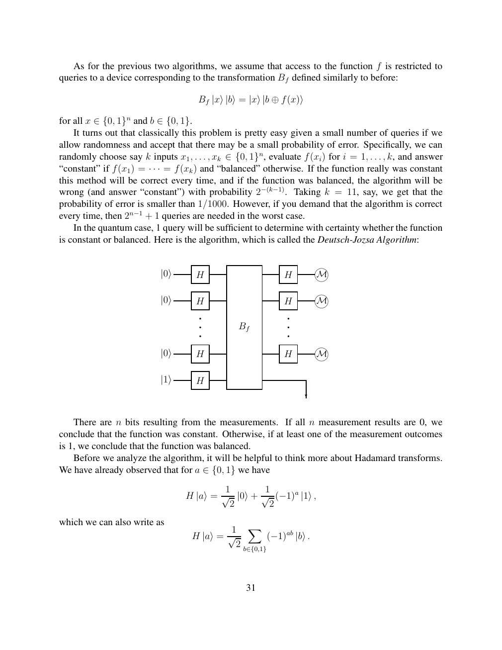
Show extracted searchable text (mathematical glyphs may differ)
As for the previous two algorithms, we assume that access to the function f is restricted to
queries to a device corresponding to the transformation Bf defined similarly to before:
Bf |x⟩|b⟩= |x⟩|b ⊕f(x)⟩
for all x and b ∈{0, 1}n ∈{0, 1}. It turns out that classically this problem is pretty easy given a small number of queries if we
allow randomness and accept that there may be a small probability of error. Specifically, we can
randomly choose say k inputs x1, . . . , xk evaluate f(xi) for i = 1, . . . , k, and answer ∈{0, 1}n,“constant” if f(x1) = = f(xk) and “balanced” otherwise. If the function really was constant · · ·this method will be correct every time, and if the function was balanced, the algorithm will be
wrong (and answer “constant”) with probability 2−(k−1). Taking k = 11, say, we get that the
probability of error is smaller than 1/1000. However, if you demand that the algorithm is correct
every time, then 2n−1 + 1 queries are needed in the worst case.
In the quantum case, 1 query will be sufficient to determine with certainty whether the function
is constant or balanced. Here is the algorithm, which is called the Deutsch-Jozsa Algorithm:
|0⟩ H H M
|0⟩ H H M
Bf
|0⟩ H H M
|1⟩ H
?
There are n bits resulting from the measurements. If all n measurement results are 0, we
conclude that the function was constant. Otherwise, if at least one of the measurement outcomes
is 1, we conclude that the function was balanced.
Before we analyze the algorithm, it will be helpful to think more about Hadamard transforms.
We have already observed that for a we have ∈{0, 1}
1 1
H |a⟩= √ 2 |0⟩+ √ 2 (−1)a |1⟩,
which we can also write as X 1
H |a⟩= √ 2 (−1)ab |b⟩.
b∈{0,1}
31
Source page 32
Direct link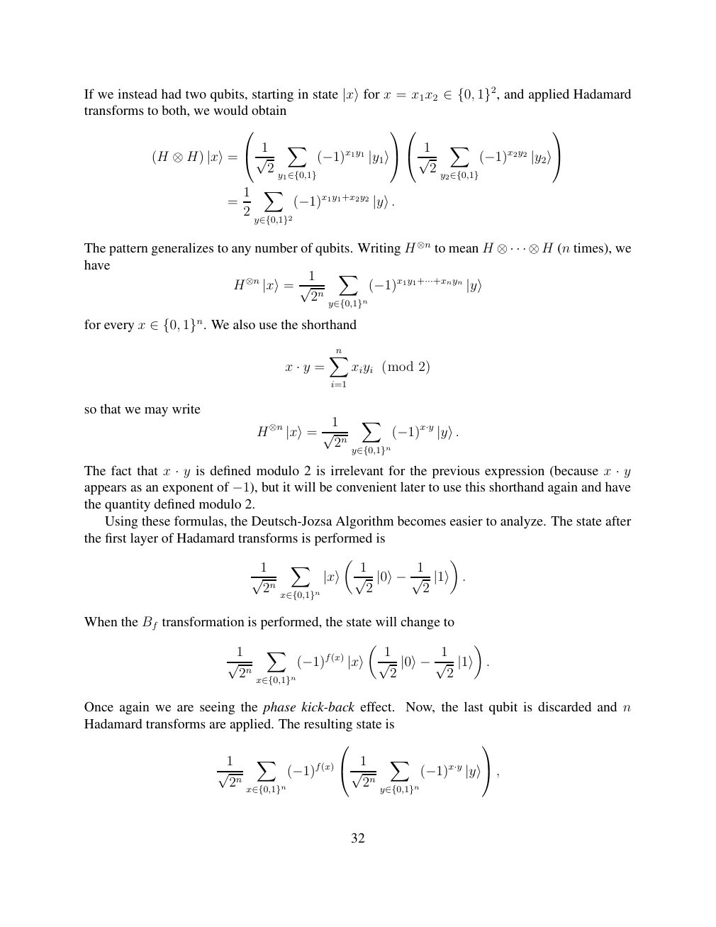
Show extracted searchable text (mathematical glyphs may differ)
If we instead had two qubits, starting in state |x⟩for x = x1x2 ∈{0, 1}2, and applied Hadamardtransforms to both, we would obtain
X X
1 1
(H ⊗H) |x⟩= √ 2 (−1)x1y1 |y1⟩ √ 2 (−1)x2y2 |y2⟩
y1∈{0,1} y2∈{0,1}
X 1
= 2 (−1)x1y1+x2y2 |y⟩.
y∈{0,1}2
The pattern generalizes to any number of qubits. Writing H ⊗n to mean H (n times), we ⊗· · · ⊗Hhave X 1
H⊗n |x⟩= √ 2n (−1)x1y1+···+xnyn |y⟩
y∈{0,1}n
for every x We also use the shorthand ∈{0, 1}n.
Xn
x · y = xiyi (mod 2)
i=1
so that we may write
X 1
H⊗n |x⟩= √ 2n (−1)x·y |y⟩.
y∈{0,1}n
The fact that x y is defined modulo 2 is irrelevant for the previous expression (because x y · ·
appears as an exponent of −1), but it will be convenient later to use this shorthand again and havethe quantity defined modulo 2.
Using these formulas, the Deutsch-Jozsa Algorithm becomes easier to analyze. The state after
the first layer of Hadamard transforms is performed is
X 1 1
. √ 2n |x⟩ √ 2 |0⟩−1√ 2 |1⟩
x∈{0,1}n
When the Bf transformation is performed, the state will change to
X 1 1
. √ 2n (−1)f(x) |x⟩ √ 2 |0⟩−1√ 2 |1⟩
x∈{0,1}n
Once again we are seeing the phase kick-back effect. Now, the last qubit is discarded and n
Hadamard transforms are applied. The resulting state is
X X
1 1
√ 2n (−1)f(x) √ 2n (−1)x·y |y⟩,
x∈{0,1}n y∈{0,1}n
32
Source page 33
Direct link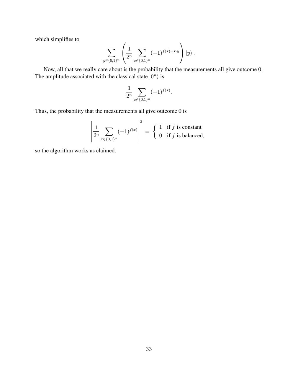
Show extracted searchable text (mathematical glyphs may differ)
which simplifies to
X X
1 2n (−1)f(x)+x·y |y⟩.
y∈{0,1}n x∈{0,1}n
Now, all that we really care about is the probability that the measurements all give outcome 0.
The amplitude associated with the classical state |0n⟩is
X 1
2n (−1)f(x).
x∈{0,1}n
Thus, the probability that the measurements all give outcome 0 is
2
X 1 1 if f is constant
= 2n (−1)f(x) 0 if f is balanced,
x∈{0,1}n
so the algorithm works as claimed.
33
⊗ Circuit walkthrough: entanglement and measurement
The Hadamard gate prepares (|0⟩ + |1⟩)/√2 on the first qubit. The controlled-NOT then creates the Bell state (|00⟩ + |11⟩)/√2. Measuring both qubits in the computational basis produces correlated 00 and 11 outcomes, each with ideal probability 1/2. This example illustrates a circuit building block; it is not a complete implementation of the surrounding algorithm.
Show runnable Qiskit example
from qiskit import QuantumCircuit
from qiskit_aer import AerSimulator

qc = QuantumCircuit(2, 2)
qc.h(0)             # Superpose the first qubit
qc.cx(0, 1)         # Entangle both qubits
qc.measure([0, 1], [0, 1])
print(qc.draw(output="text"))
result = AerSimulator().run(qc, shots=1024).result()
print(result.get_counts())  # Approximately 00 and 11
Install qiskit and qiskit-aer locally to execute this code. The diagram is a static circuit illustration, not a browser-based simulator.