Math fidelity: The original PDF page is displayed as a high-resolution image so that equations, bra–ket notation, matrix layouts and circuit diagrams remain exactly as in the source. The expandable text layer is for searching and may not reproduce every mathematical glyph.
Source page 126
Direct link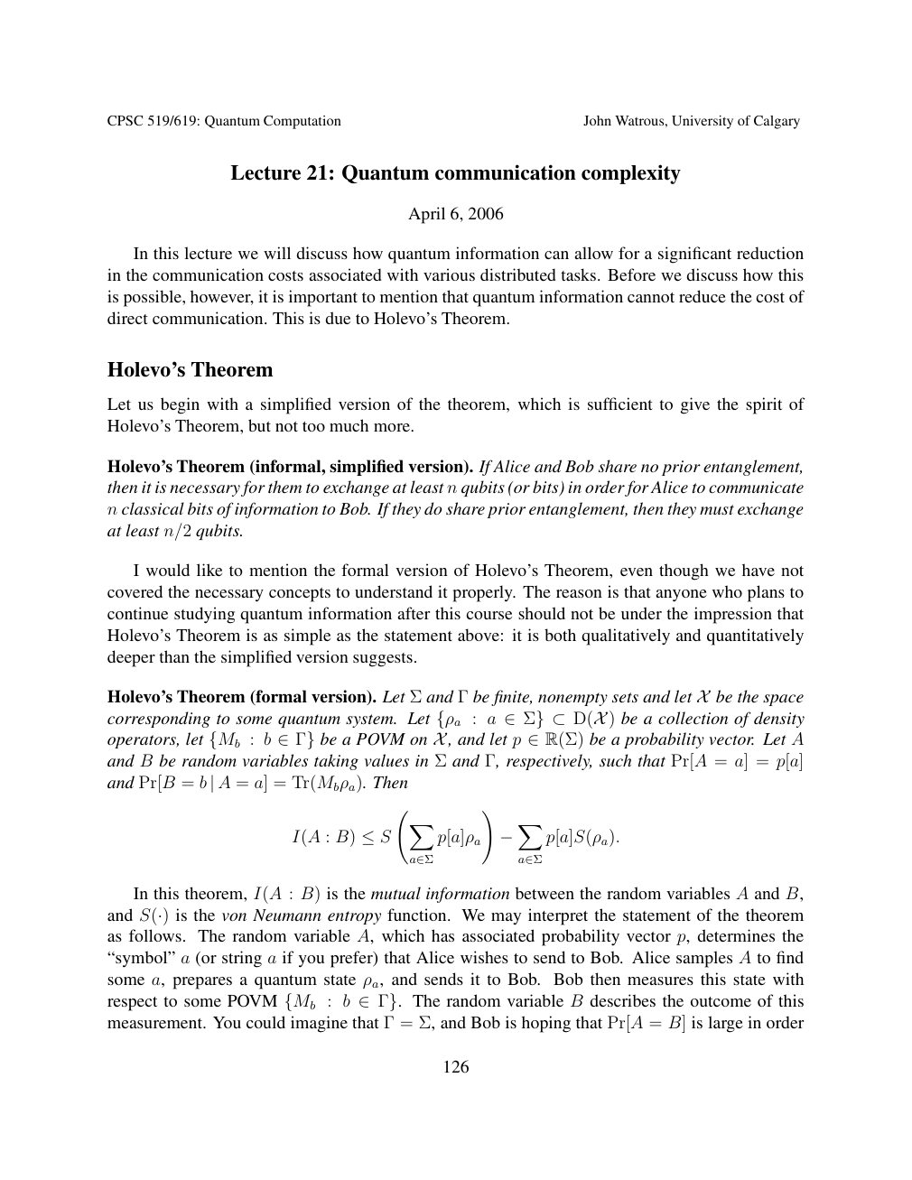
Show extracted searchable text (mathematical glyphs may differ)
CPSC 519/619: Quantum Computation John Watrous, University of Calgary
Lecture 21: Quantum communication complexity
April 6, 2006
In this lecture we will discuss how quantum information can allow for a significant reduction
in the communication costs associated with various distributed tasks. Before we discuss how this
is possible, however, it is important to mention that quantum information cannot reduce the cost of
direct communication. This is due to Holevo’s Theorem.
Holevo’s Theorem
Let us begin with a simplified version of the theorem, which is sufficient to give the spirit of
Holevo’s Theorem, but not too much more.
Holevo’s Theorem (informal, simplified version). If Alice and Bob share no prior entanglement,
then it is necessary for them to exchange at least n qubits (or bits) in order for Alice to communicate
n classical bits of information to Bob. If they do share prior entanglement, then they must exchange
at least n/2 qubits.
I would like to mention the formal version of Holevo’s Theorem, even though we have not
covered the necessary concepts to understand it properly. The reason is that anyone who plans to
continue studying quantum information after this course should not be under the impression that
Holevo’s Theorem is as simple as the statement above: it is both qualitatively and quantitatively
deeper than the simplified version suggests.
Holevo’s Theorem (formal version). Let Σ and Γ be finite, nonempty sets and let be the space X
corresponding to some quantum system. Let {ρa : a ∈Σ} ⊂D(X ) be a collection of density
operators, let {Mb : b ∈Γ} be a POVM on X , and let p ∈R(Σ) be a probability vector. Let Aand B be random variables taking values in Σ and Γ, respectively, such that Pr[A = a] = p[a]
and Pr[B = b | A = a] = Tr(Mbρa). Then
!
X X
I(A : B) ≤S p[a]ρa − p[a]S(ρa).
a∈Σ a∈Σ
In this theorem, I(A : B) is the mutual information between the random variables A and B,
and is the von Neumann entropy function. We may interpret the statement of the theorem S(·)as follows. The random variable A, which has associated probability vector p, determines the
“symbol” a (or string a if you prefer) that Alice wishes to send to Bob. Alice samples A to find
some a, prepares a quantum state ρa, and sends it to Bob. Bob then measures this state with
respect to some POVM : b The random variable B describes the outcome of this {Mb ∈Γ}.measurement. You could imagine that Γ = Σ, and Bob is hoping that Pr[A = B] is large in order
126
Source page 127
Direct link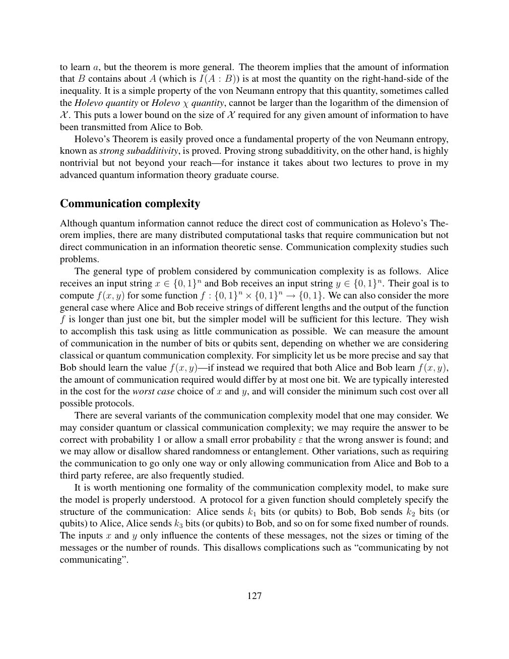
Show extracted searchable text (mathematical glyphs may differ)
to learn a, but the theorem is more general. The theorem implies that the amount of information
that B contains about A (which is I(A : B)) is at most the quantity on the right-hand-side of the
inequality. It is a simple property of the von Neumann entropy that this quantity, sometimes called
the Holevo quantity or Holevo χ quantity, cannot be larger than the logarithm of the dimension of
. This puts a lower bound on the size of required for any given amount of information to haveX Xbeen transmitted from Alice to Bob.
Holevo’s Theorem is easily proved once a fundamental property of the von Neumann entropy,
known as strong subadditivity, is proved. Proving strong subadditivity, on the other hand, is highly
nontrivial but not beyond your reach—for instance it takes about two lectures to prove in my
advanced quantum information theory graduate course.
Communication complexity
Although quantum information cannot reduce the direct cost of communication as Holevo’s The-
orem implies, there are many distributed computational tasks that require communication but not
direct communication in an information theoretic sense. Communication complexity studies such
problems.
The general type of problem considered by communication complexity is as follows. Alice
receives an input string x and Bob receives an input string y Their goal is to ∈{0, 1}n ∈{0, 1}n.compute f(x, y) for some function f : We can also consider the more {0, 1}n × {0, 1}n →{0, 1}.general case where Alice and Bob receive strings of different lengths and the output of the function
f is longer than just one bit, but the simpler model will be sufficient for this lecture. They wish
to accomplish this task using as little communication as possible. We can measure the amount
of communication in the number of bits or qubits sent, depending on whether we are considering
classical or quantum communication complexity. For simplicity let us be more precise and say that
Bob should learn the value f(x, y)—if instead we required that both Alice and Bob learn f(x, y),
the amount of communication required would differ by at most one bit. We are typically interested
in the cost for the worst case choice of x and y, and will consider the minimum such cost over all
possible protocols.
There are several variants of the communication complexity model that one may consider. We
may consider quantum or classical communication complexity; we may require the answer to be
correct with probability 1 or allow a small error probability ε that the wrong answer is found; and
we may allow or disallow shared randomness or entanglement. Other variations, such as requiring
the communication to go only one way or only allowing communication from Alice and Bob to a
third party referee, are also frequently studied.
It is worth mentioning one formality of the communication complexity model, to make sure
the model is properly understood. A protocol for a given function should completely specify the
structure of the communication: Alice sends k1 bits (or qubits) to Bob, Bob sends k2 bits (or
qubits) to Alice, Alice sends k3 bits (or qubits) to Bob, and so on for some fixed number of rounds.
The inputs x and y only influence the contents of these messages, not the sizes or timing of the
messages or the number of rounds. This disallows complications such as “communicating by not
communicating”.
127
Source page 128
Direct link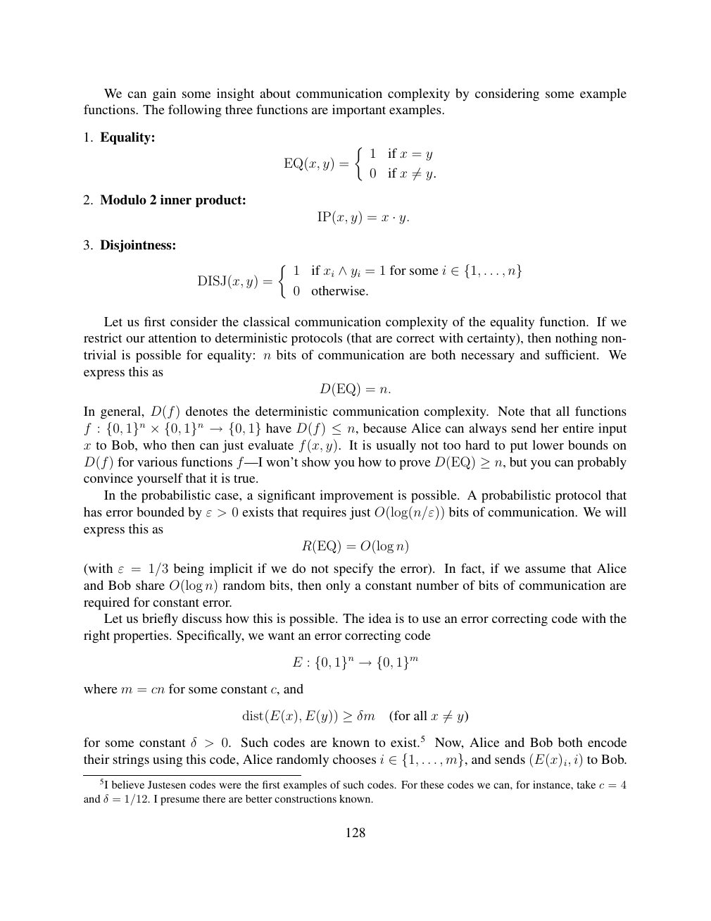
Show extracted searchable text (mathematical glyphs may differ)
We can gain some insight about communication complexity by considering some example
functions. The following three functions are important examples.
1. Equality:
1 if x = y
EQ(x, y) =
0 if x y. ̸=
2. Modulo 2 inner product:
IP(x, y) = x · y.
3. Disjointness:
1 if xi = 1 for some i . . . , DISJ(x, y) = ∧yi ∈{1, n}
0 otherwise.
Let us first consider the classical communication complexity of the equality function. If we
restrict our attention to deterministic protocols (that are correct with certainty), then nothing non-
trivial is possible for equality: n bits of communication are both necessary and sufficient. We
express this as
D(EQ) = n.
In general, D(f) denotes the deterministic communication complexity. Note that all functions
f : have D(f) because Alice can always send her entire input {0, 1}n × {0, 1}n →{0, 1} ≤n,x to Bob, who then can just evaluate f(x, y). It is usually not too hard to put lower bounds on
D(f) for various functions f—I won’t show you how to prove D(EQ) ≥n, but you can probablyconvince yourself that it is true.
In the probabilistic case, a significant improvement is possible. A probabilistic protocol that
has error bounded by ε > 0 exists that requires just O(log(n/ε)) bits of communication. We will
express this as
R(EQ) = O(log n)
(with ε = 1/3 being implicit if we do not specify the error). In fact, if we assume that Alice
and Bob share O(log n) random bits, then only a constant number of bits of communication are
required for constant error.
Let us briefly discuss how this is possible. The idea is to use an error correcting code with the
right properties. Specifically, we want an error correcting code
E : {0, 1}n →{0, 1}m
where m = cn for some constant c, and
dist(E(x), E(y)) (for all x y) ≥δm ̸=
for some constant δ > 0. Such codes are known to exist.5 Now, Alice and Bob both encode
their strings using this code, Alice randomly chooses i . . . , and sends (E(x)i, i) to Bob. ∈{1, m},
5I believe Justesen codes were the first examples of such codes. For these codes we can, for instance, take c = 4
and δ = 1/12. I presume there are better constructions known.
128
Source page 129
Direct link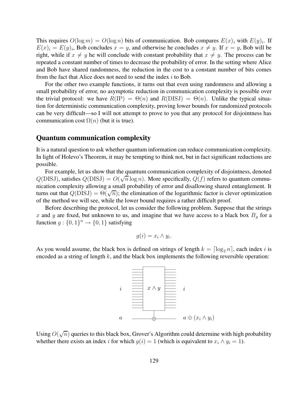
Show extracted searchable text (mathematical glyphs may differ)
This requires O(log m) = O(log n) bits of communication. Bob compares E(x)i with E(y)i. If
E(x)i = E(y)i, Bob concludes x = y, and otherwise he concludes x y. If x = y, Bob will be ̸=right, while if x y he will conclude with constant probability that x y. The process can be ̸= ̸=repeated a constant number of times to decrease the probability of error. In the setting where Alice
and Bob have shared randomness, the reduction in the cost to a constant number of bits comes
from the fact that Alice does not need to send the index i to Bob.
For the other two example functions, it turns out that even using randomness and allowing a
small probability of error, no asymptotic reduction in communication complexity is possible over
the trivial protocol: we have R(IP) = Θ(n) and R(DISJ) = Θ(n). Unlike the typical situa-
tion for deterministic communication complexity, proving lower bounds for randomized protocols
can be very difficult—so I will not attempt to prove to you that any protocol for disjointness has
communication cost Ω(n) (but it is true).
Quantum communication complexity
It is a natural question to ask whether quantum information can reduce communication complexity.
In light of Holevo’s Theorem, it may be tempting to think not, but in fact significant reductions are
possible.
For example, let us show that the quantum communication complexity of disjointness, denoted
Q(DISJ), satisfies Q(DISJ) = O(√n log n). More specifically, Q(f) refers to quantum commu-
nication complexity allowing a small probability of error and disallowing shared entanglement. It
turns out that Q(DISJ) = Θ(√n); the elimination of the logarithmic factor is clever optimization
of the method we will see, while the lower bound requires a rather difficult proof.
Before describing the protocol, let us consider the following problem. Suppose that the strings
x and y are fixed, but unknown to us, and imagine that we have access to a black box Bg for a
function g : satisfying {0, 1}n →{0, 1}
g(i) = xi ∧yi.
As you would assume, the black box is defined on strings of length k = each index i is ⌈log2 n⌉,encoded as a string of length k, and the black box implements the following reversible operation:
i x ∧y i
a a ⊕(xi ∧yi)
Using O(√n) queries to this black box, Grover’s Algorithm could determine with high probability
whether there exists an index i for which g(i) = 1 (which is equivalent to xi = 1). ∧yi
129
Source page 130
Direct link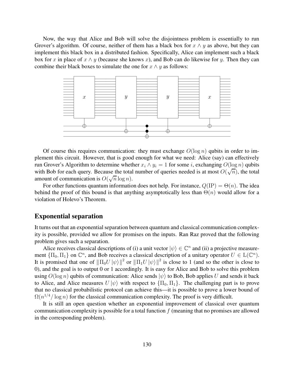
Show extracted searchable text (mathematical glyphs may differ)
Now, the way that Alice and Bob will solve the disjointness problem is essentially to run
Grover’s algorithm. Of course, neither of them has a black box for x as above, but they can ∧yimplement this black box in a distributed fashion. Specifically, Alice can implement such a black
box for x in place of x (because she knows x), and Bob can do likewise for y. Then they can ∧ycombine their black boxes to simulate the one for x as follows: ∧y
x y y x
Of course this requires communication: they must exchange O(log n) qubits in order to im-
plement this circuit. However, that is good enough for what we need: Alice (say) can effectively
run Grover’s Algorithm to determine whether xi = 1 for some i, exchanging O(log n) qubits ∧yiwith Bob for each query. Because the total number of queries needed is at most O(√n), the total
amount of communication is O(√n log n).
For other functions quantum information does not help. For instance, Q(IP) = Θ(n). The idea
behind the proof of this bound is that anything asymptotically less than Θ(n) would allow for a
violation of Holevo’s Theorem.
Exponential separation
It turns out that an exponential separation between quantum and classical communication complex-
ity is possible, provided we allow for promises on the inputs. Ran Raz proved that the following
problem gives such a separation.
Alice receives classical descriptions of (i) a unit vector |ψ⟩∈Cn and (ii) a projective measure-ment on Cn, and Bob receives a classical description of a unitary operator U {Π0, Π1} ∈L(Cn).It is promised that one of or is close to 1 (and so the other is close to ∥Π0U |ψ⟩∥2 ∥Π1U |ψ⟩∥20), and the goal is to output 0 or 1 accordingly. It is easy for Alice and Bob to solve this problem
U and sends it backusing O(log n) qubits of communication: Alice sends |ψ⟩to Bob, Bob applies
to Alice, and Alice measures U |ψ⟩with respect to {Π0, Π1}. The challenging part is to provethat no classical probabilistic protocol can achieve this—it is possible to prove a lower bound of
Ω(n1/4/ log n) for the classical communication complexity. The proof is very difficult.
It is still an open question whether an exponential improvement of classical over quantum
communication complexity is possible for a total function f (meaning that no promises are allowed
in the corresponding problem).
130
Source page 131
Direct link
Show extracted searchable text (mathematical glyphs may differ)
Quantum fingerprinting
Finally, I would like to mention a variant of the communication complexity model where it is
possible to prove an exponential separation between quantum and classical complexities for a total
function (i.e., not a promise problem). It is a very weak model called the simultaneous message
passing model. As before, Alice receives an input string x and Bob receives y, but now Alice and
Bob cannot communicate with one another at all. Instead, they must both send a single message to
a third party, called the referee. The referee does not receive any input, but is required to give the
output of the function f based on the messages received from Alice and Bob.
One can consider several variants of this model—we will compare the classical probabilistic
model with the quantum model, where the referee is allowed a small probability of error in both
cases. No shared randomness or entanglement will be permitted between Alice and Bob. (If we
do allow shared randomness or entanglement, the example to be considered no longer gives an
interesting separation between quantum and classical.)
The separation will be for the equality function. If we write R∥(f) to denote the randomized
communication complexity of f in the simultaneous message passing model, then we have
R∥(EQ) = Θ(√n).
In contrast, using a similar notation for the quantum case, we have
Q∥(EQ) = O(log n).
The technique that establishes that Q∥(EQ) = O(log n) is called quantum fingerprinting. The
idea is that Alice will prepare a small quantum state |ψx⟩given x, and Bob will prepare |ψy⟩given
y. We want that each |ψx⟩is a quantum state on a number of qubits that is logarithmic in n, but so
that |ψx⟩and |ψy⟩are very different when x ̸= y. The state |ψx⟩is a “fingerprint” of x—it doesnot contain enough information for someone to recover x from it, but it can be used to distinguish
x from another string y with a different fingerprint. The referee will then attempt to check whether
the fingerprints |ψx⟩and |ψy⟩are the same or different. Of course it is not possible to come up with states x that form an orthonor- {|ψx⟩: ∈{0, 1}n}mal set, because this would require that the fingerprints are too large: at least n qubits. So instead
what we will do is to make them pairwise “almost orthogonal”: should be small when- |⟨ψx|ψy⟩|ever x y. We can do this using exactly the same kind of error correcting codes we discussed in ̸=the first part of the lecture. Specifically, we let
Xm 1
|ψx⟩= √m |i⟩|E(x)i⟩.
i=1
Then, assuming dist(E(x), E(y)) for x y, we have Replacing ≥δm ̸= |⟨ψx|ψy⟩| ≤1 −δ.
|ψx⟩with some constant number of copies of |ψx⟩allows this bound on the inner product to bedecreased to an arbitrarily small constant. The number of qubits required for these fingerprints is
small: O(log n) qubits.
Now, how can the referee determine whether is small? You’ve already |ψx⟩= |ψy⟩or |⟨ψx|ψy⟩|answered this question (in a slightly simplified form) in question 3 of homework assignment 1. In
that question, you were asked to consider this circuit:
131
Source page 132
Direct link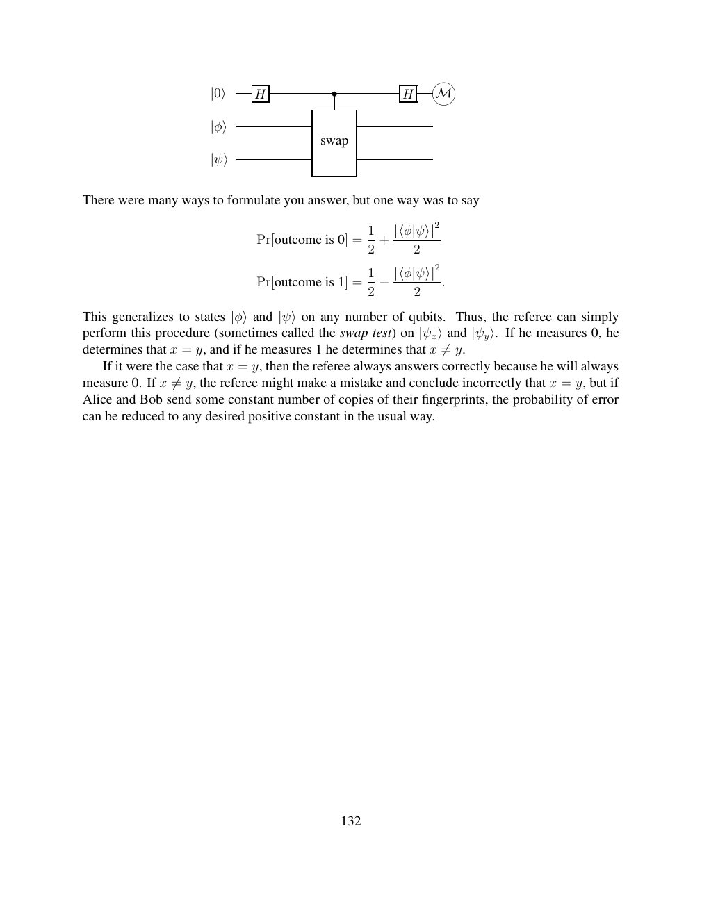
Show extracted searchable text (mathematical glyphs may differ)
|0⟩ H H M
|φ⟩ swap
|ψ⟩
There were many ways to formulate you answer, but one way was to say
1 Pr[outcome is 0] = + |⟨φ|ψ⟩|2
2 2
1
Pr[outcome is 1] = . 2 −|⟨φ|ψ⟩|22
This generalizes to states |φ⟩and |ψ⟩on any number of qubits. Thus, the referee can simply
perform this procedure (sometimes called the swap test) on |ψx⟩and |ψy⟩. If he measures 0, hedetermines that x = y, and if he measures 1 he determines that x y. ̸= If it were the case that x = y, then the referee always answers correctly because he will always
measure 0. If x y, the referee might make a mistake and conclude incorrectly that x = y, but if ̸=Alice and Bob send some constant number of copies of their fingerprints, the probability of error
can be reduced to any desired positive constant in the usual way.
132
⊗ Circuit walkthrough: entanglement and measurement
The Hadamard gate prepares (|0⟩ + |1⟩)/√2 on the first qubit. The controlled-NOT then creates the Bell state (|00⟩ + |11⟩)/√2. Measuring both qubits in the computational basis produces correlated 00 and 11 outcomes, each with ideal probability 1/2. This example illustrates a circuit building block; it is not a complete implementation of the surrounding algorithm.
Show runnable Qiskit example
from qiskit import QuantumCircuit
from qiskit_aer import AerSimulator

qc = QuantumCircuit(2, 2)
qc.h(0)             # Superpose the first qubit
qc.cx(0, 1)         # Entangle both qubits
qc.measure([0, 1], [0, 1])
print(qc.draw(output="text"))
result = AerSimulator().run(qc, shots=1024).result()
print(result.get_counts())  # Approximately 00 and 11
Install qiskit and qiskit-aer locally to execute this code. The diagram is a static circuit illustration, not a browser-based simulator.