Math fidelity: The original PDF page is displayed as a high-resolution image so that equations, bra–ket notation, matrix layouts and circuit diagrams remain exactly as in the source. The expandable text layer is for searching and may not reproduce every mathematical glyph.
Source page 133
Direct link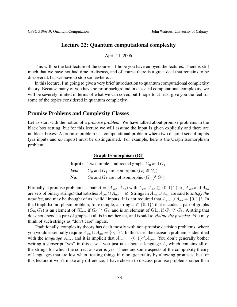
Show extracted searchable text (mathematical glyphs may differ)
CPSC 519/619: Quantum Computation John Watrous, University of Calgary
Lecture 22: Quantum computational complexity
April 11, 2006
This will be the last lecture of the course—I hope you have enjoyed the lectures. There is still
much that we have not had time to discuss, and of course there is a great deal that remains to be
discovered, but we have to stop somewhere. . .
In this lecture, I’m going to give a very brief introduction to quantum computational complexity
theory. Because many of you have no prior background in classical computational complexity, we
will be severely limited in terms of what we can cover, but I hope to at least give you the feel for
some of the topics considered in quantum complexity.
Promise Problems and Complexity Classes
Let us start with the notion of a promise problem. We have talked about promise problems in the
black box setting, but for this lecture we will assume the input is given explicitly and there are
no black boxes. A promise problem is a computational problem where two disjoint sets of inputs
(yes inputs and no inputs) must be distinguished. For example, here is the Graph Isomorphism
problem:
Graph Isomorphism (GI)
Input: Two simple, undirected graphs G0 and G1.
Yes: G0 and G1 are isomorphic (G0 ∼= G1).
No: G0 and G1 are not isomorphic (G0 ̸∼= G1).
Formally, a promise problem is a pair A = (Ayes, Ano) with Ayes, Ano Ayes and Ano ⊆{0, 1}∗(i.e.,are sets of binary strings) that satisfies Ayes = ∅. Strings in Ayes are said to satisfy the ∩Ano ∪Anopromise, and may be thought of as “valid” inputs. It is not required that Ayes = In ∪Ano {0, 1}∗.the Graph Isomorphism problem, for example, a string x encodes a pair of graphs ∈{0, 1}∗that
(G0, G1) is an element of GIyes if G0 ∼= G1, and is an element of GIno if G0 ̸∼= G1. A string thatdoes not encode a pair of graphs at all is in neither set, and is said to violate the promise. You may
think of such strings as “don’t care” inputs.
Traditionally, complexity theory has dealt mostly with non-promise decision problems, where
you would essentially require Ayes = In this case, the decision problem is identified ∪Ano {0, 1}∗.with the language Ayes, and it is implicit that Ano = You don’t generally bother {0, 1}∗\Ayes.writing a subscript “yes” in this case—you just talk about a language A, which contains all of
the strings for which the correct answer is yes. There are some aspects of the complexity theory
of languages that are lost when treating things in more generality by allowing promises, but for
this lecture it won’t make any difference. I have chosen to discuss promise problems rather than
133
Source page 134
Direct link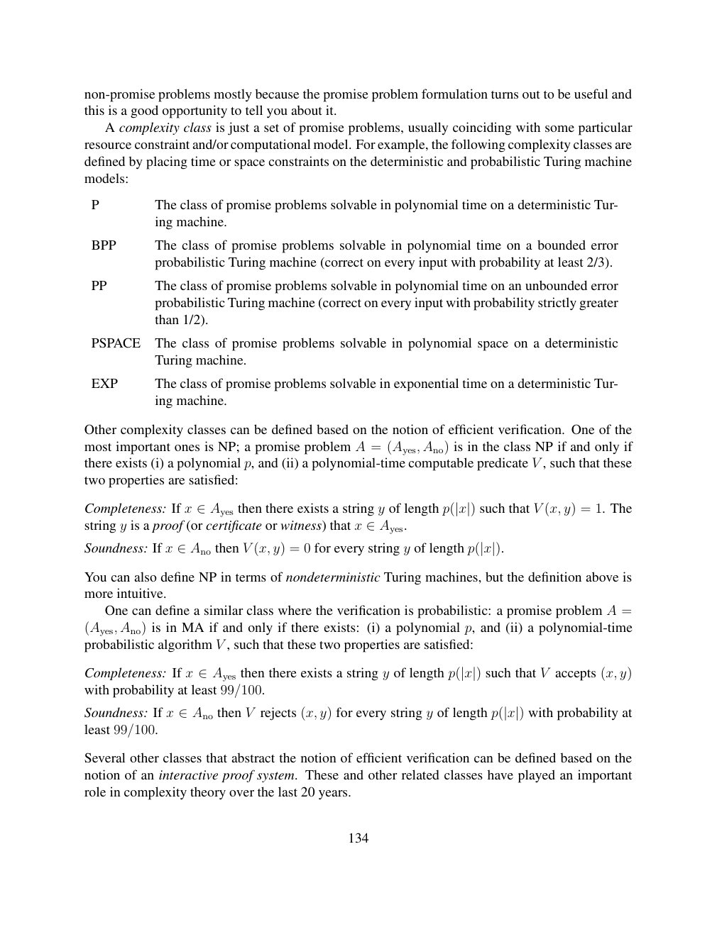
Show extracted searchable text (mathematical glyphs may differ)
non-promise problems mostly because the promise problem formulation turns out to be useful and
this is a good opportunity to tell you about it.
A complexity class is just a set of promise problems, usually coinciding with some particular
resource constraint and/or computational model. For example, the following complexity classes are
defined by placing time or space constraints on the deterministic and probabilistic Turing machine
models:
P The class of promise problems solvable in polynomial time on a deterministic Tur-
ing machine.
BPP The class of promise problems solvable in polynomial time on a bounded error
probabilistic Turing machine (correct on every input with probability at least 2/3).
PP The class of promise problems solvable in polynomial time on an unbounded error
probabilistic Turing machine (correct on every input with probability strictly greater
than 1/2).
PSPACE The class of promise problems solvable in polynomial space on a deterministic
Turing machine.
EXP The class of promise problems solvable in exponential time on a deterministic Tur-
ing machine.
Other complexity classes can be defined based on the notion of efficient verification. One of the
most important ones is NP; a promise problem A = (Ayes, Ano) is in the class NP if and only if
there exists (i) a polynomial p, and (ii) a polynomial-time computable predicate V , such that these
two properties are satisfied:
Completeness: If x then there exists a string y of length such that V (x, y) = 1. The ∈Ayes p(|x|)
string y is a proof (or certificate or witness) that x ∈Ayes.
Soundness: If x then V (x, y) = 0 for every string y of length ∈Ano p(|x|).
You can also define NP in terms of nondeterministic Turing machines, but the definition above is
more intuitive.
One can define a similar class where the verification is probabilistic: a promise problem A =
(Ayes, Ano) is in MA if and only if there exists: (i) a polynomial p, and (ii) a polynomial-time
probabilistic algorithm V , such that these two properties are satisfied:
Completeness: If x then there exists a string y of length such that V accepts (x, y) ∈Ayes p(|x|)with probability at least 99/100.
Soundness: If x then V rejects (x, y) for every string y of length with probability at ∈Ano p(|x|)least 99/100.
Several other classes that abstract the notion of efficient verification can be defined based on the
notion of an interactive proof system. These and other related classes have played an important
role in complexity theory over the last 20 years.
134
Source page 135
Direct link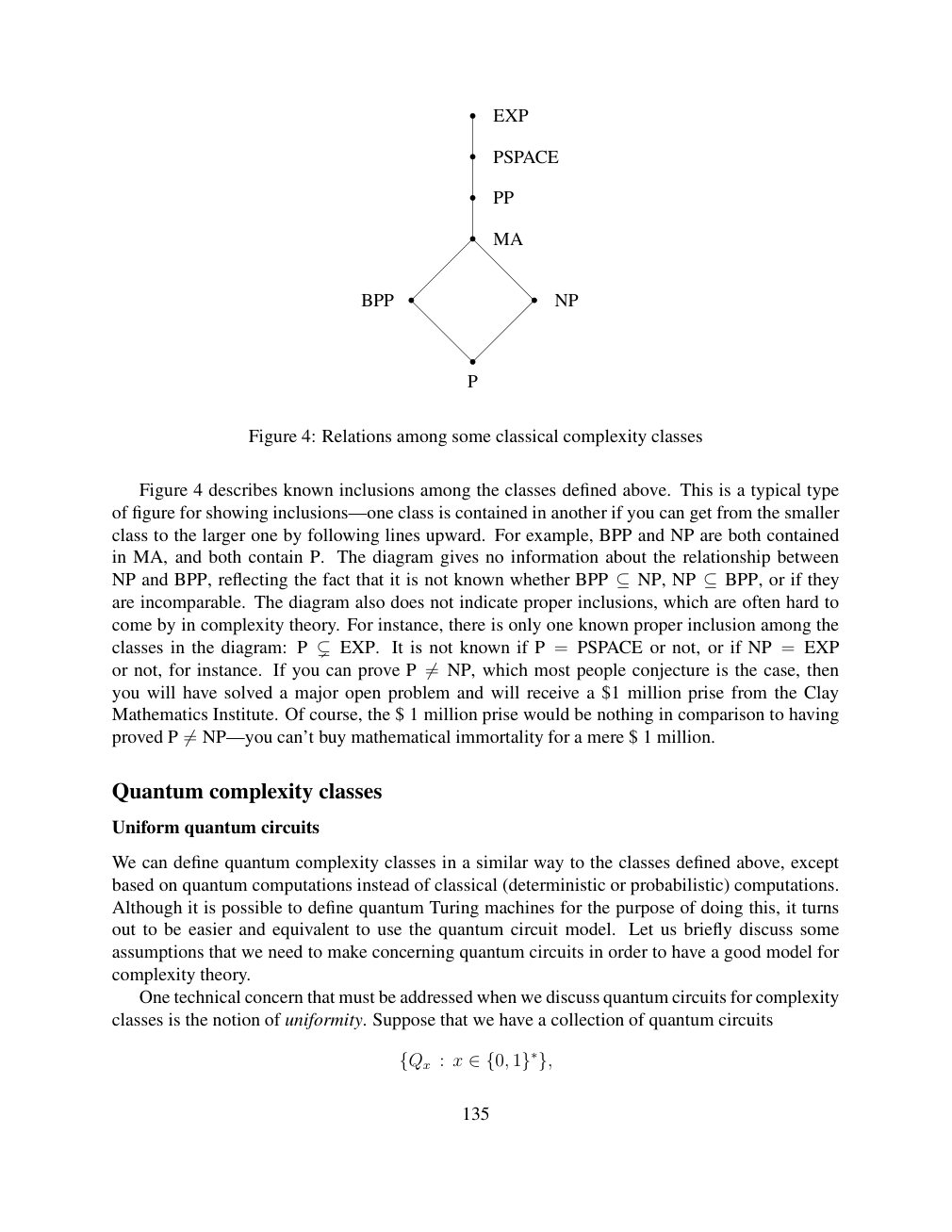
Show extracted searchable text (mathematical glyphs may differ)
EXP
PSPACE
PP
MA
BPP NP
P
Figure 4: Relations among some classical complexity classes
Figure 4 describes known inclusions among the classes defined above. This is a typical type
of figure for showing inclusions—one class is contained in another if you can get from the smaller
class to the larger one by following lines upward. For example, BPP and NP are both contained
in MA, and both contain P. The diagram gives no information about the relationship between
NP and BPP, reflecting the fact that it is not known whether BPP ⊆NP, NP ⊆BPP, or if theyare incomparable. The diagram also does not indicate proper inclusions, which are often hard to
come by in complexity theory. For instance, there is only one known proper inclusion among the
classes in the diagram: P ⊊EXP. It is not known if P = PSPACE or not, or if NP = EXP
or not, for instance. If you can prove P NP, which most people conjecture is the case, then ̸=you will have solved a major open problem and will receive a $1 million prise from the Clay
Mathematics Institute. Of course, the $ 1 million prise would be nothing in comparison to having
proved P NP—you can’t buy mathematical immortality for a mere $ 1 million. ̸=
Quantum complexity classes
Uniform quantum circuits
We can define quantum complexity classes in a similar way to the classes defined above, except
based on quantum computations instead of classical (deterministic or probabilistic) computations.
Although it is possible to define quantum Turing machines for the purpose of doing this, it turns
out to be easier and equivalent to use the quantum circuit model. Let us briefly discuss some
assumptions that we need to make concerning quantum circuits in order to have a good model for
complexity theory.
One technical concern that must be addressed when we discuss quantum circuits for complexity
classes is the notion of uniformity. Suppose that we have a collection of quantum circuits
{Qx : x ∈{0, 1}∗},
135
Source page 136
Direct link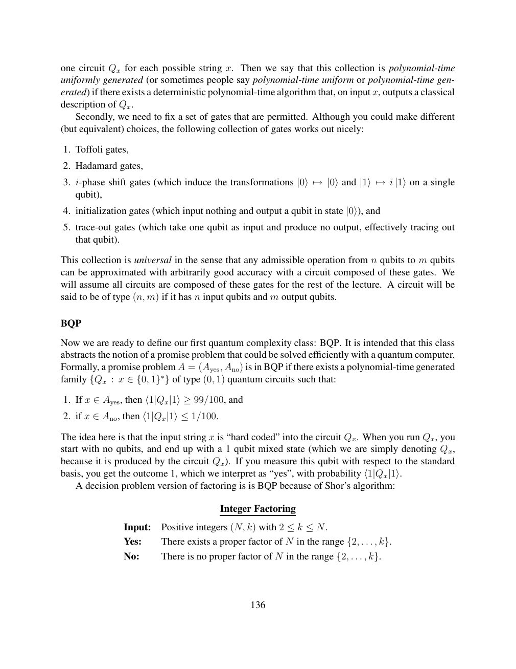
Show extracted searchable text (mathematical glyphs may differ)
one circuit Qx for each possible string x. Then we say that this collection is polynomial-time
uniformly generated (or sometimes people say polynomial-time uniform or polynomial-time gen-
erated) if there exists a deterministic polynomial-time algorithm that, on input x, outputs a classical
description of Qx.
Secondly, we need to fix a set of gates that are permitted. Although you could make different
(but equivalent) choices, the following collection of gates works out nicely:
1. Toffoli gates,
2. Hadamard gates,
3. i-phase shift gates (which induce the transformations |0⟩7→|0⟩and |1⟩7→i |1⟩on a single qubit),
4. initialization gates (which input nothing and output a qubit in state |0⟩), and
5. trace-out gates (which take one qubit as input and produce no output, effectively tracing out
that qubit).
This collection is universal in the sense that any admissible operation from n qubits to m qubits
can be approximated with arbitrarily good accuracy with a circuit composed of these gates. We
will assume all circuits are composed of these gates for the rest of the lecture. A circuit will be
said to be of type (n, m) if it has n input qubits and m output qubits.
BQP
Now we are ready to define our first quantum complexity class: BQP. It is intended that this class
abstracts the notion of a promise problem that could be solved efficiently with a quantum computer.
Formally, a promise problem A = (Ayes, Ano) is in BQP if there exists a polynomial-time generated
family : x of type (0, 1) quantum circuits such that: {Qx ∈{0, 1}∗}
1. If x ∈Ayes, then ⟨1|Qx|1⟩≥99/100, and
2. if x ∈Ano, then ⟨1|Qx|1⟩≤1/100.
The idea here is that the input string x is “hard coded” into the circuit Qx. When you run Qx, you
start with no qubits, and end up with a 1 qubit mixed state (which we are simply denoting Qx,
because it is produced by the circuit Qx). If you measure this qubit with respect to the standard
basis, you get the outcome 1, which we interpret as “yes”, with probability ⟨1|Qx|1⟩. A decision problem version of factoring is is BQP because of Shor’s algorithm:
Integer Factoring
Input: Positive integers (N, k) with 2 ≤k ≤N.
Yes: There exists a proper factor of N in the range . . . , {2, k}.
No: There is no proper factor of N in the range . . . , {2, k}.
136
Source page 137
Direct link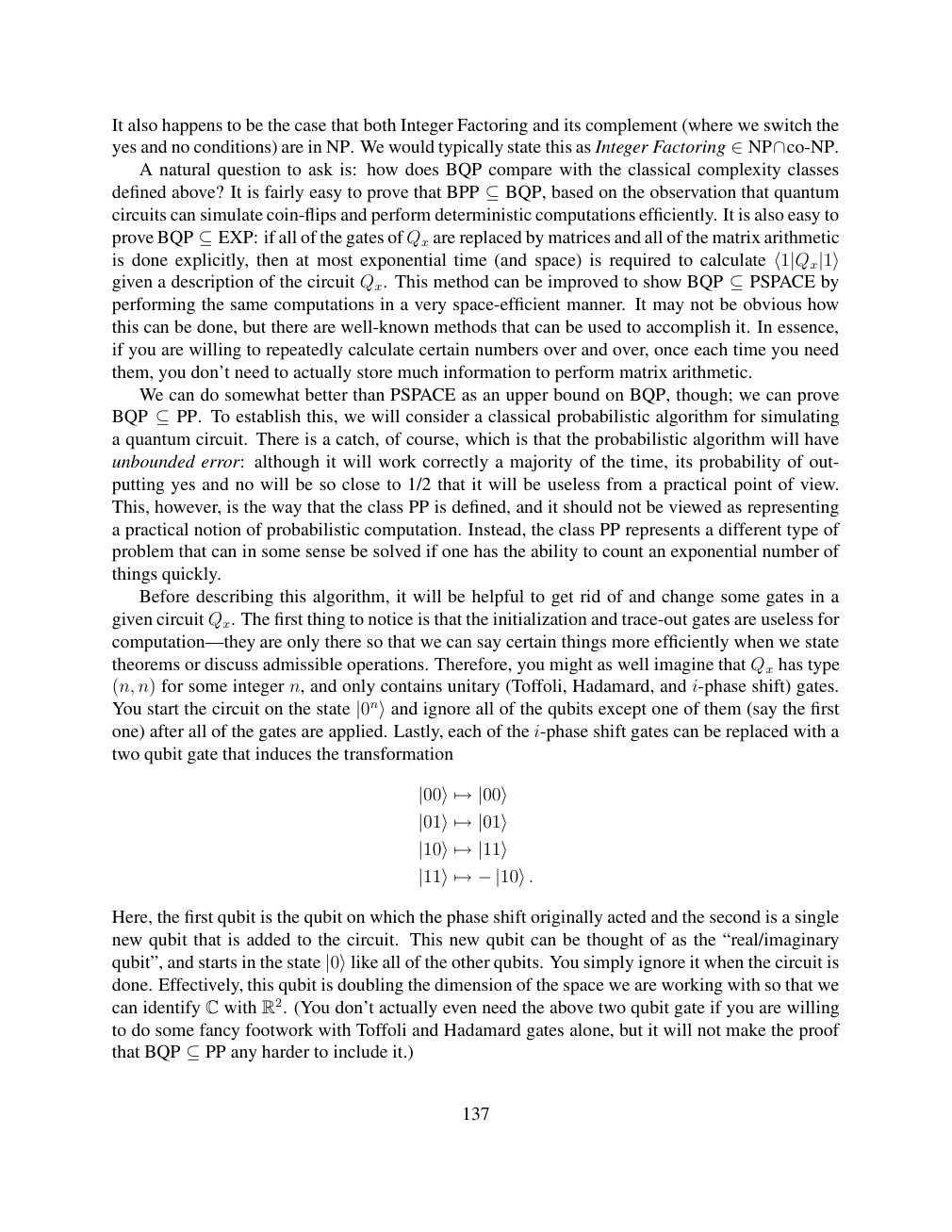
Show extracted searchable text (mathematical glyphs may differ)
It also happens to be the case that both Integer Factoring and its complement (where we switch the
yes and no conditions) are in NP. We would typically state this as Integer Factoring ∈NP∩co-NP. A natural question to ask is: how does BQP compare with the classical complexity classes
defined above? It is fairly easy to prove that BPP ⊆BQP, based on the observation that quantumcircuits can simulate coin-flips and perform deterministic computations efficiently. It is also easy to
Qx are replaced by matrices and all of the matrix arithmeticprove BQP ⊆EXP: if all of the gates ofis done explicitly, then at most exponential time (and space) is required to calculate ⟨1|Qx|1⟩
given a description of the circuit Qx. This method can be improved to show BQP ⊆PSPACE byperforming the same computations in a very space-efficient manner. It may not be obvious how
this can be done, but there are well-known methods that can be used to accomplish it. In essence,
if you are willing to repeatedly calculate certain numbers over and over, once each time you need
them, you don’t need to actually store much information to perform matrix arithmetic.
We can do somewhat better than PSPACE as an upper bound on BQP, though; we can prove
BQP ⊆PP. To establish this, we will consider a classical probabilistic algorithm for simulatinga quantum circuit. There is a catch, of course, which is that the probabilistic algorithm will have
unbounded error: although it will work correctly a majority of the time, its probability of out-
putting yes and no will be so close to 1/2 that it will be useless from a practical point of view.
This, however, is the way that the class PP is defined, and it should not be viewed as representing
a practical notion of probabilistic computation. Instead, the class PP represents a different type of
problem that can in some sense be solved if one has the ability to count an exponential number of
things quickly.
Before describing this algorithm, it will be helpful to get rid of and change some gates in a
given circuit Qx. The first thing to notice is that the initialization and trace-out gates are useless for
computation—they are only there so that we can say certain things more efficiently when we state
theorems or discuss admissible operations. Therefore, you might as well imagine that Qx has type
(n, n) for some integer n, and only contains unitary (Toffoli, Hadamard, and i-phase shift) gates.
You start the circuit on the state |0n⟩and ignore all of the qubits except one of them (say the firstone) after all of the gates are applied. Lastly, each of the i-phase shift gates can be replaced with a
two qubit gate that induces the transformation
|00⟩7→|00⟩
|01⟩7→|01⟩
|10⟩7→|11⟩
|11⟩7→−|10⟩.
Here, the first qubit is the qubit on which the phase shift originally acted and the second is a single
new qubit that is added to the circuit. This new qubit can be thought of as the “real/imaginary
qubit”, and starts in the state |0⟩like all of the other qubits. You simply ignore it when the circuit isdone. Effectively, this qubit is doubling the dimension of the space we are working with so that we
can identify C with R2. (You don’t actually even need the above two qubit gate if you are willing
to do some fancy footwork with Toffoli and Hadamard gates alone, but it will not make the proof
that BQP ⊆PP any harder to include it.)
137
Source page 138
Direct link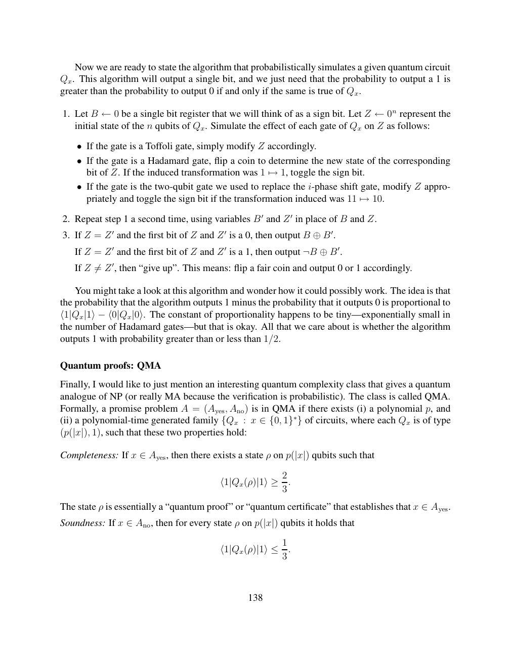
Show extracted searchable text (mathematical glyphs may differ)
Now we are ready to state the algorithm that probabilistically simulates a given quantum circuit
Qx. This algorithm will output a single bit, and we just need that the probability to output a 1 is
greater than the probability to output 0 if and only if the same is true of Qx.
1. Let B be a single bit register that we will think of as a sign bit. Let Z represent the ←0 ←0n initial state of the n qubits of Qx. Simulate the effect of each gate of Qx on Z as follows:
If the gate is a Toffoli gate, simply modify Z accordingly. •
If the gate is a Hadamard gate, flip a coin to determine the new state of the corresponding •
bit of Z. If the induced transformation was 1 7→1, toggle the sign bit.
If the gate is the two-qubit gate we used to replace the i-phase shift gate, modify Z appro- •
priately and toggle the sign bit if the transformation induced was 11 7→10.
2. Repeat step 1 a second time, using variables B′ and Z′ in place of B and Z.
3. If Z = Z′ and the first bit of Z and Z′ is a 0, then output B ⊕B′.
If Z = Z′ and the first bit of Z and Z′ is a 1, then output ¬B ⊕B′.
If Z Z′, then “give up”. This means: flip a fair coin and output 0 or 1 accordingly. ̸=
You might take a look at this algorithm and wonder how it could possibly work. The idea is that
the probability that the algorithm outputs 1 minus the probability that it outputs 0 is proportional to
⟨1|Qx|1⟩−⟨0|Qx|0⟩. The constant of proportionality happens to be tiny—exponentially small inthe number of Hadamard gates—but that is okay. All that we care about is whether the algorithm
outputs 1 with probability greater than or less than 1/2.
Quantum proofs: QMA
Finally, I would like to just mention an interesting quantum complexity class that gives a quantum
analogue of NP (or really MA because the verification is probabilistic). The class is called QMA.
Formally, a promise problem A = (Ayes, Ano) is in QMA if there exists (i) a polynomial p, and
(ii) a polynomial-time generated family : x of circuits, where each Qx is of type {Qx ∈{0, 1}∗} 1), such that these two properties hold:(p(|x|),
ρ on qubits such thatCompleteness: If x ∈Ayes, then there exists a state p(|x|)
⟨1|Qx(ρ)|1⟩≥23.
The state ρ is essentially a “quantum proof” or “quantum certificate” that establishes that x ∈Ayes.
ρ on qubits it holds thatSoundness: If x ∈Ano, then for every state p(|x|)
⟨1|Qx(ρ)|1⟩≤13.
138
Source page 139
Direct link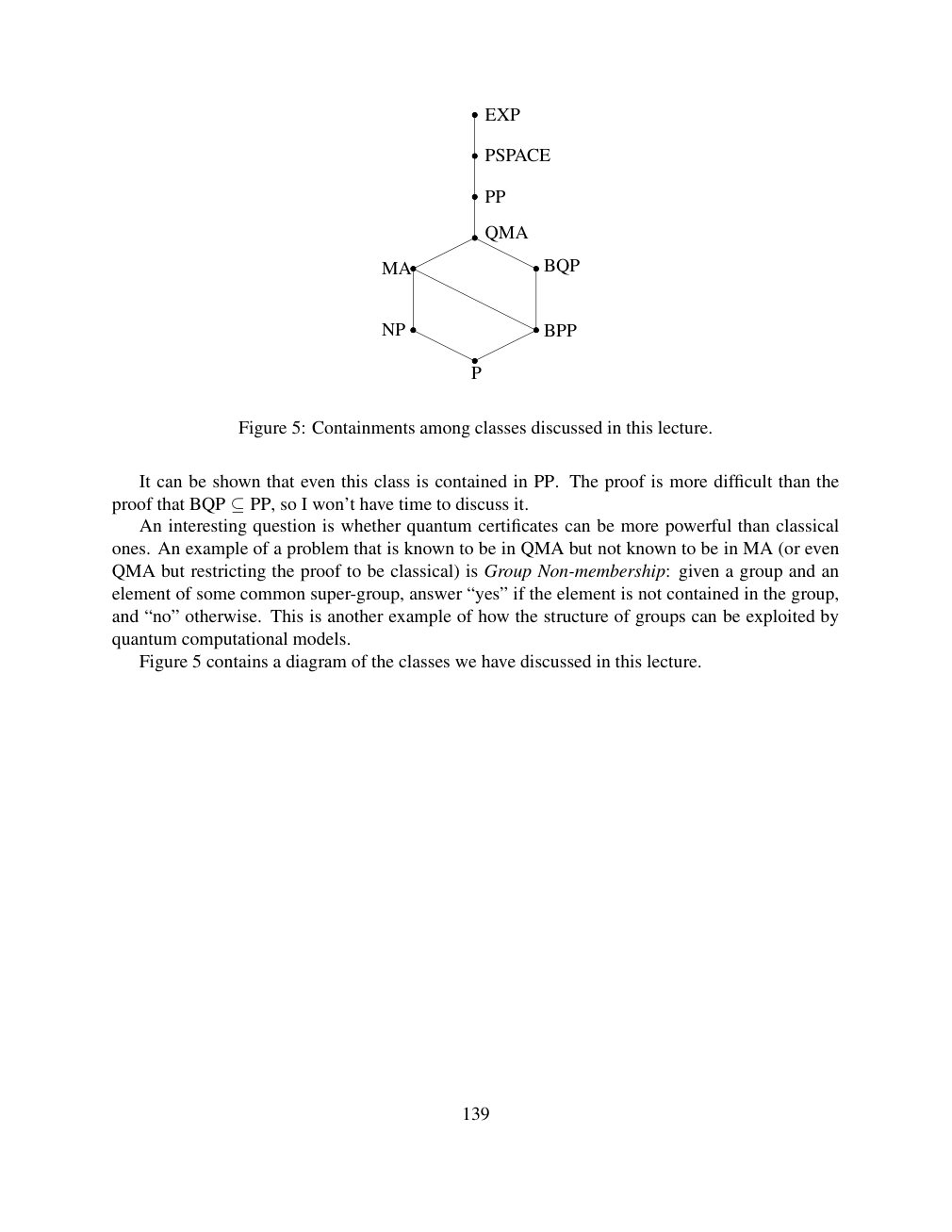
Show extracted searchable text (mathematical glyphs may differ)
EXP
PSPACE
PP
QMA
MA BQP
NP BPP
P
Figure 5: Containments among classes discussed in this lecture.
It can be shown that even this class is contained in PP. The proof is more difficult than the
proof that BQP ⊆PP, so I won’t have time to discuss it. An interesting question is whether quantum certificates can be more powerful than classical
ones. An example of a problem that is known to be in QMA but not known to be in MA (or even
QMA but restricting the proof to be classical) is Group Non-membership: given a group and an
element of some common super-group, answer “yes” if the element is not contained in the group,
and “no” otherwise. This is another example of how the structure of groups can be exploited by
quantum computational models.
Figure 5 contains a diagram of the classes we have discussed in this lecture.
139
⊗ Circuit walkthrough: entanglement and measurement
The Hadamard gate prepares (|0⟩ + |1⟩)/√2 on the first qubit. The controlled-NOT then creates the Bell state (|00⟩ + |11⟩)/√2. Measuring both qubits in the computational basis produces correlated 00 and 11 outcomes, each with ideal probability 1/2. This example illustrates a circuit building block; it is not a complete implementation of the surrounding algorithm.
Show runnable Qiskit example
from qiskit import QuantumCircuit
from qiskit_aer import AerSimulator

qc = QuantumCircuit(2, 2)
qc.h(0)             # Superpose the first qubit
qc.cx(0, 1)         # Entangle both qubits
qc.measure([0, 1], [0, 1])
print(qc.draw(output="text"))
result = AerSimulator().run(qc, shots=1024).result()
print(result.get_counts())  # Approximately 00 and 11
Install qiskit and qiskit-aer locally to execute this code. The diagram is a static circuit illustration, not a browser-based simulator.