Math fidelity: The original PDF page is displayed as a high-resolution image so that equations, bra–ket notation, matrix layouts and circuit diagrams remain exactly as in the source. The expandable text layer is for searching and may not reproduce every mathematical glyph.
Source page 39
Direct link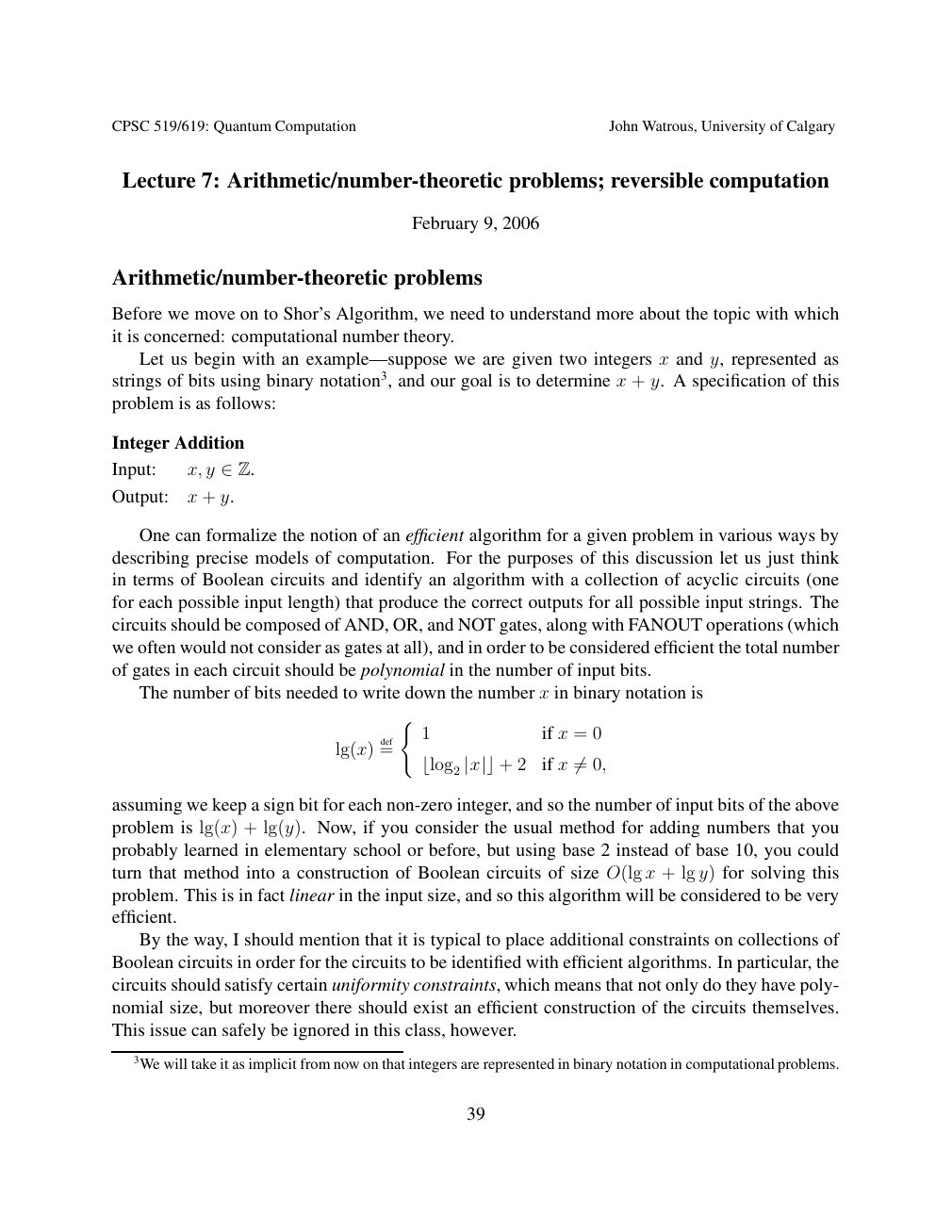
Show extracted searchable text (mathematical glyphs may differ)
CPSC 519/619: Quantum Computation John Watrous, University of Calgary
Lecture 7: Arithmetic/number-theoretic problems; reversible computation
February 9, 2006
Arithmetic/number-theoretic problems
Before we move on to Shor’s Algorithm, we need to understand more about the topic with which
it is concerned: computational number theory.
Let us begin with an example—suppose we are given two integers x and y, represented as
strings of bits using binary notation3, and our goal is to determine x + y. A specification of this
problem is as follows:
Integer Addition
Input: x, y ∈Z.
Output: x + y.
One can formalize the notion of an efficient algorithm for a given problem in various ways by
describing precise models of computation. For the purposes of this discussion let us just think
in terms of Boolean circuits and identify an algorithm with a collection of acyclic circuits (one
for each possible input length) that produce the correct outputs for all possible input strings. The
circuits should be composed of AND, OR, and NOT gates, along with FANOUT operations (which
we often would not consider as gates at all), and in order to be considered efficient the total number
of gates in each circuit should be polynomial in the number of input bits.
The number of bits needed to write down the number x in binary notation is
(
1 if x = 0
lg(x) def=
2 if x 0, ⌊log2 |x|⌋+ ̸=
assuming we keep a sign bit for each non-zero integer, and so the number of input bits of the above
problem is lg(x) + lg(y). Now, if you consider the usual method for adding numbers that you
probably learned in elementary school or before, but using base 2 instead of base 10, you could
turn that method into a construction of Boolean circuits of size O(lg x + lg y) for solving this
problem. This is in fact linear in the input size, and so this algorithm will be considered to be very
efficient.
By the way, I should mention that it is typical to place additional constraints on collections of
Boolean circuits in order for the circuits to be identified with efficient algorithms. In particular, the
circuits should satisfy certain uniformity constraints, which means that not only do they have poly-
nomial size, but moreover there should exist an efficient construction of the circuits themselves.
This issue can safely be ignored in this class, however.
3We will take it as implicit from now on that integers are represented in binary notation in computational problems.
39
Source page 40
Direct link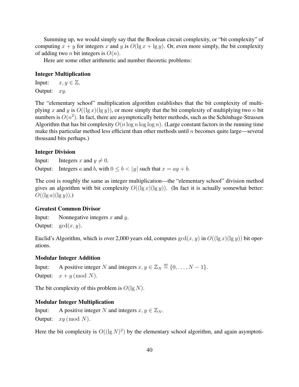
Show extracted searchable text (mathematical glyphs may differ)
Summing up, we would simply say that the Boolean circuit complexity, or “bit complexity” of
computing x + y for integers x and y is O(lg x + lg y). Or, even more simply, the bit complexity
of adding two n bit integers is O(n).
Here are some other arithmetic and number theoretic problems:
Integer Multiplication
Input: x, y ∈Z.
Output: xy.
The “elementary school” multiplication algorithm establishes that the bit complexity of multi-
plying x and y is O((lg x)(lg y)), or more simply that the bit complexity of multiplying two n bit
numbers is O(n2). In fact, there are asymptotically better methods, such as the Sch¨onhage-Strassen
Algorithm that has bit complexity O(n log n log log n). (Large constant factors in the running time
make this particular method less efficient than other methods until n becomes quite large—several
thousand bits perhaps.)
Integer Division
Input: Integers x and y 0. ̸=
Output: Integers a and b, with 0 < such that x = ay + b. ≤b |y|
The cost is roughly the same as integer multiplication—the “elementary school” division method
gives an algorithm with bit complexity O((lg x)(lg y)). (In fact it is actually somewhat better:
O((lg a)(lg y)).)
Greatest Common Divisor
Input: Nonnegative integers x and y.
Output: gcd(x, y).
Euclid’s Algorithm, which is over 2,000 years old, computes gcd(x, y) in O((lg x)(lg y)) bit oper-
ations.
Modular Integer Addition
Input: A positive integer N and integers x, y def= . . . , N ∈ZN {0, −1}.
Output: x + y (mod N).
The bit complexity of this problem is O(lg N).
Modular Integer Multiplication
Input: A positive integer N and integers x, y ∈ZN.
Output: xy (mod N).
Here the bit complexity is O((lg N)2) by the elementary school algorithm, and again asymptoti-
40
Source page 41
Direct link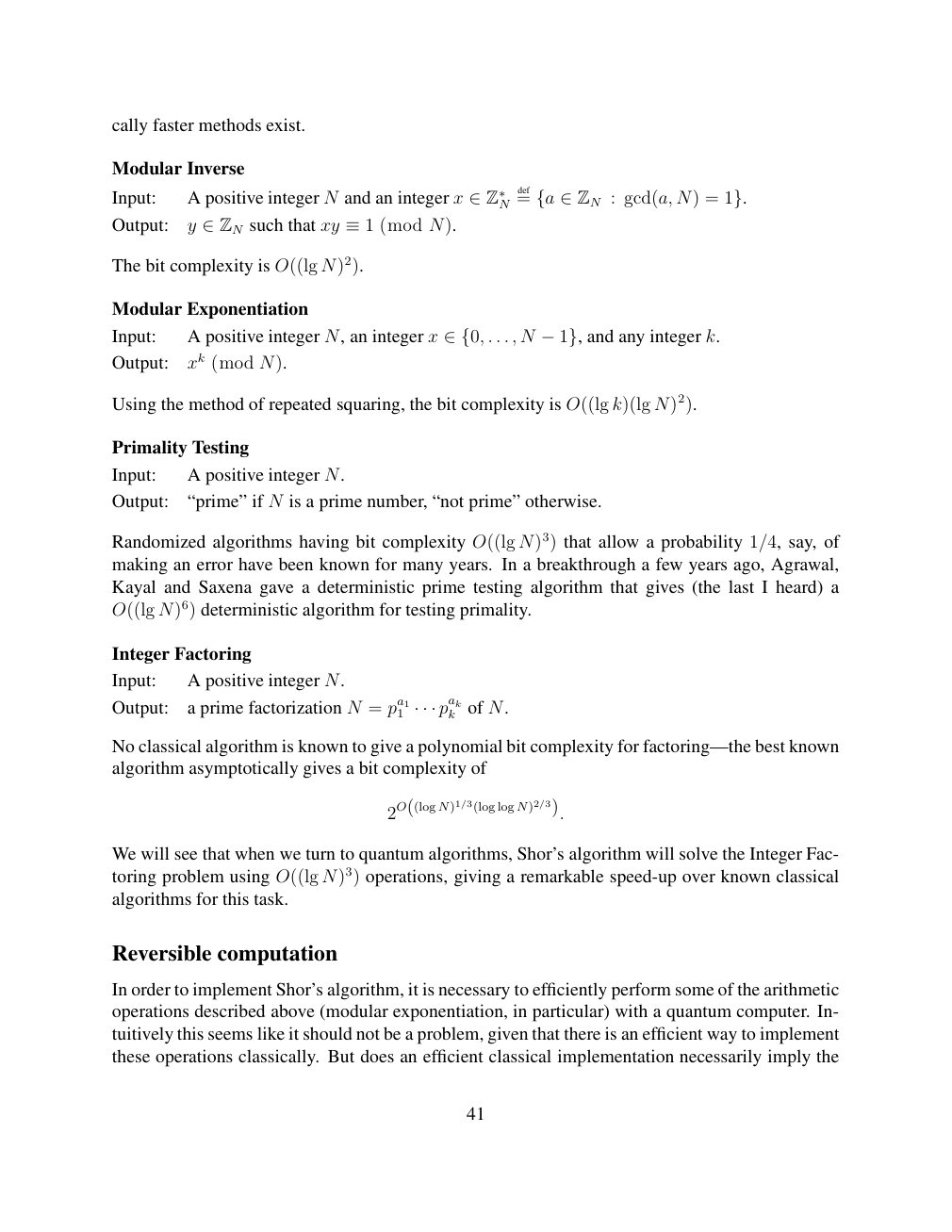
Show extracted searchable text (mathematical glyphs may differ)
cally faster methods exist.
Modular Inverse
N def=Input: A positive integer N and an integer x ∈Z∗ {a ∈ZN : gcd(a, N) = 1}.
Output: y such that xy (mod N). ∈ZN ≡1
The bit complexity is O((lg N)2).
Modular Exponentiation
Input: A positive integer N, an integer x . . . , N and any integer k. ∈{0, −1},
Output: xk (mod N).
Using the method of repeated squaring, the bit complexity is O((lg k)(lg N)2).
Primality Testing
Input: A positive integer N.
Output: “prime” if N is a prime number, “not prime” otherwise.
Randomized algorithms having bit complexity O((lg N)3) that allow a probability 1/4, say, of
making an error have been known for many years. In a breakthrough a few years ago, Agrawal,
Kayal and Saxena gave a deterministic prime testing algorithm that gives (the last I heard) a
O((lg N)6) deterministic algorithm for testing primality.
Integer Factoring
Input: A positive integer N.
Output: a prime factorization N = pa11 pakk of N. · · ·
No classical algorithm is known to give a polynomial bit complexity for factoring—the best known
algorithm asymptotically gives a bit complexity of
2O((log N)1/3(log log N)2/3).
We will see that when we turn to quantum algorithms, Shor’s algorithm will solve the Integer Fac-
toring problem using O((lg N)3) operations, giving a remarkable speed-up over known classical
algorithms for this task.
Reversible computation
In order to implement Shor’s algorithm, it is necessary to efficiently perform some of the arithmetic
operations described above (modular exponentiation, in particular) with a quantum computer. In-
tuitively this seems like it should not be a problem, given that there is an efficient way to implement
these operations classically. But does an efficient classical implementation necessarily imply the
41
Source page 42
Direct link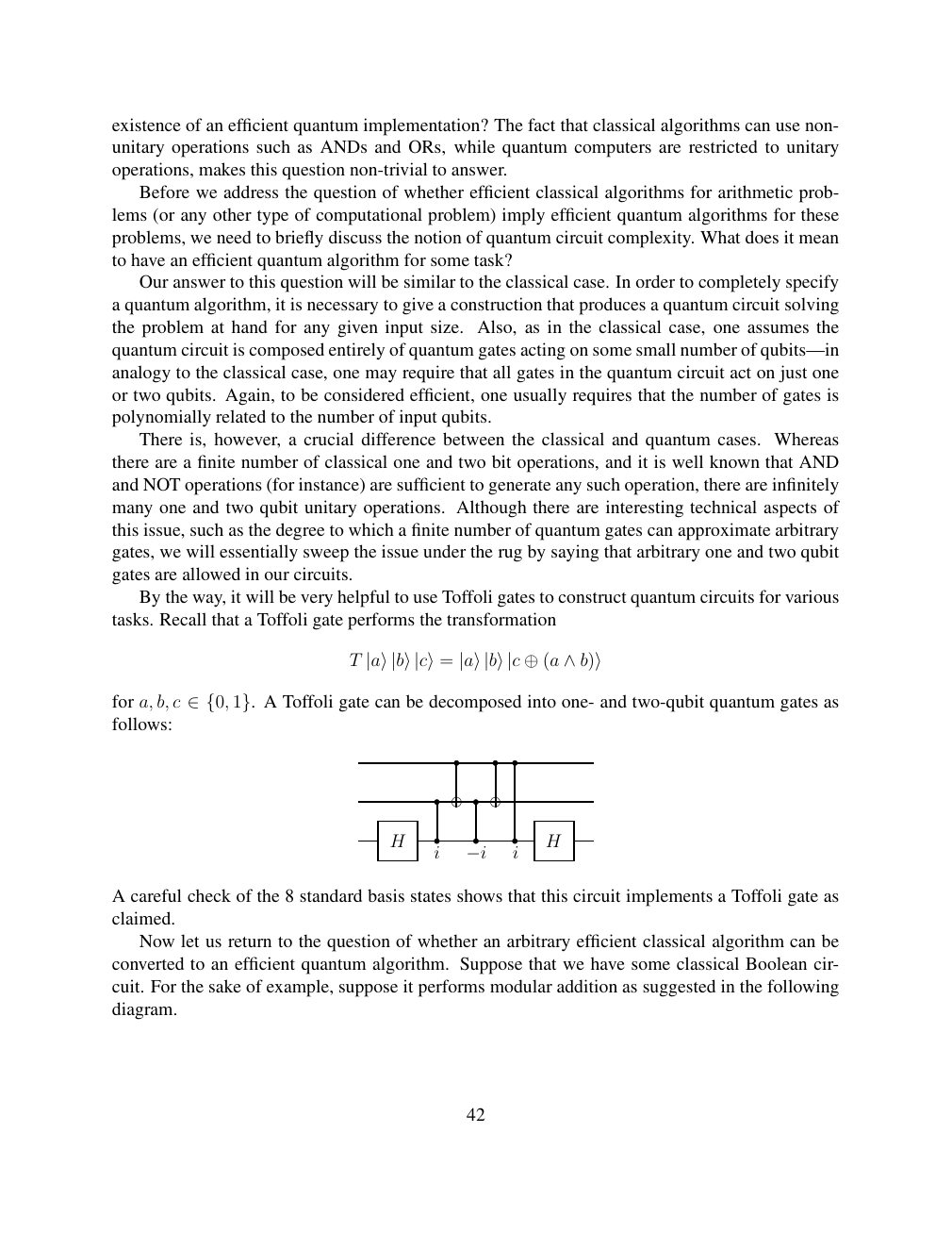
Show extracted searchable text (mathematical glyphs may differ)
existence of an efficient quantum implementation? The fact that classical algorithms can use non-
unitary operations such as ANDs and ORs, while quantum computers are restricted to unitary
operations, makes this question non-trivial to answer.
Before we address the question of whether efficient classical algorithms for arithmetic prob-
lems (or any other type of computational problem) imply efficient quantum algorithms for these
problems, we need to briefly discuss the notion of quantum circuit complexity. What does it mean
to have an efficient quantum algorithm for some task?
Our answer to this question will be similar to the classical case. In order to completely specify
a quantum algorithm, it is necessary to give a construction that produces a quantum circuit solving
the problem at hand for any given input size. Also, as in the classical case, one assumes the
quantum circuit is composed entirely of quantum gates acting on some small number of qubits—in
analogy to the classical case, one may require that all gates in the quantum circuit act on just one
or two qubits. Again, to be considered efficient, one usually requires that the number of gates is
polynomially related to the number of input qubits.
There is, however, a crucial difference between the classical and quantum cases. Whereas
there are a finite number of classical one and two bit operations, and it is well known that AND
and NOT operations (for instance) are sufficient to generate any such operation, there are infinitely
many one and two qubit unitary operations. Although there are interesting technical aspects of
this issue, such as the degree to which a finite number of quantum gates can approximate arbitrary
gates, we will essentially sweep the issue under the rug by saying that arbitrary one and two qubit
gates are allowed in our circuits.
By the way, it will be very helpful to use Toffoli gates to construct quantum circuits for various
tasks. Recall that a Toffoli gate performs the transformation
T |a⟩|b⟩|c⟩= |a⟩|b⟩|c ⊕(a ∧b)⟩
for a, b, c A Toffoli gate can be decomposed into one- and two-qubit quantum gates as ∈{0, 1}.follows:
H H
i −i i
A careful check of the 8 standard basis states shows that this circuit implements a Toffoli gate as
claimed.
Now let us return to the question of whether an arbitrary efficient classical algorithm can be
converted to an efficient quantum algorithm. Suppose that we have some classical Boolean cir-
cuit. For the sake of example, suppose it performs modular addition as suggested in the following
diagram.
42
Source page 43
Direct link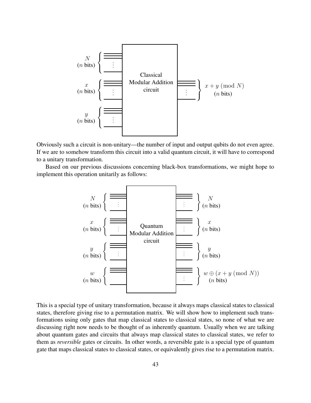
Show extracted searchable text (mathematical glyphs may differ)
N
(n bits)
Classical
Modular Addition x x + y (mod N) circuit (n bits) (n bits)
y
(n bits)
Obviously such a circuit is non-unitary—the number of input and output qubits do not even agree.
If we are to somehow transform this circuit into a valid quantum circuit, it will have to correspond
to a unitary transformation.
Based on our previous discussions concerning black-box transformations, we might hope to
implement this operation unitarily as follows:
( )
N N
(n bits) (n bits)
( )
x x
Quantum (n bits) (n bits)
Modular Addition
( circuit )
y y
(n bits) (n bits)
( )
w w ⊕(x + y (mod N)) (n bits) (n bits)
This is a special type of unitary transformation, because it always maps classical states to classical
states, therefore giving rise to a permutation matrix. We will show how to implement such trans-
formations using only gates that map classical states to classical states, so none of what we are
discussing right now needs to be thought of as inherently quantum. Usually when we are talking
about quantum gates and circuits that always map classical states to classical states, we refer to
them as reversible gates or circuits. In other words, a reversible gate is a special type of quantum
gate that maps classical states to classical states, or equivalently gives rise to a permutation matrix.
43
Source page 44
Direct link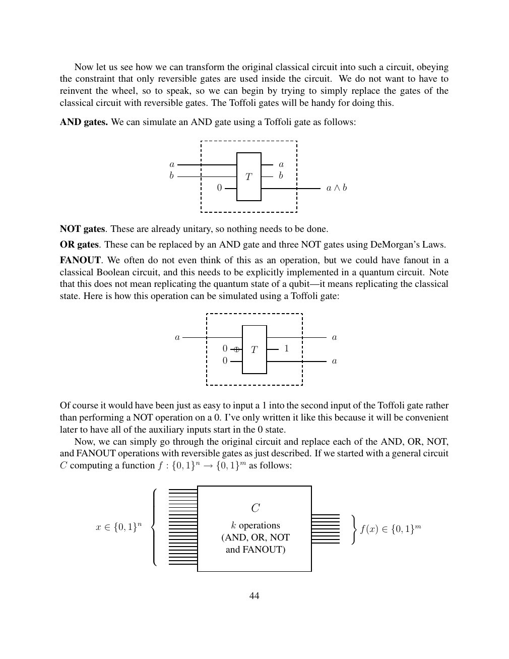
Show extracted searchable text (mathematical glyphs may differ)
Now let us see how we can transform the original classical circuit into such a circuit, obeying
the constraint that only reversible gates are used inside the circuit. We do not want to have to
reinvent the wheel, so to speak, so we can begin by trying to simply replace the gates of the
classical circuit with reversible gates. The Toffoli gates will be handy for doing this.
AND gates. We can simulate an AND gate using a Toffoli gate as follows:
a a
b T b
0 a ∧b
NOT gates. These are already unitary, so nothing needs to be done.
OR gates. These can be replaced by an AND gate and three NOT gates using DeMorgan’s Laws.
FANOUT. We often do not even think of this as an operation, but we could have fanout in a
classical Boolean circuit, and this needs to be explicitly implemented in a quantum circuit. Note
that this does not mean replicating the quantum state of a qubit—it means replicating the classical
state. Here is how this operation can be simulated using a Toffoli gate:
a a
0 T 1
0 a
Of course it would have been just as easy to input a 1 into the second input of the Toffoli gate rather
than performing a NOT operation on a 0. I’ve only written it like this because it will be convenient
later to have all of the auxiliary inputs start in the 0 state.
Now, we can simply go through the original circuit and replace each of the AND, OR, NOT,
and FANOUT operations with reversible gates as just described. If we started with a general circuit
C computing a function f : as follows: {0, 1}n →{0, 1}m
C )
x k operations f(x) ∈{0, 1}n ∈{0, 1}m (AND, OR, NOT and FANOUT)
44
Source page 45
Direct link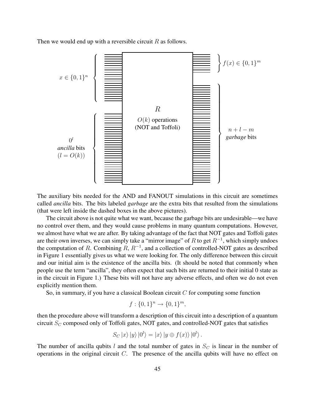
Show extracted searchable text (mathematical glyphs may differ)
Then we would end up with a reversible circuit R as follows.
)
f(x) ∈{0, 1}m
x ∈{0, 1}n R O(k) operations (NOT and Toffoli) n + l −m garbage bits 0l ancilla bits (l = O(k))
The auxiliary bits needed for the AND and FANOUT simulations in this circuit are sometimes
called ancilla bits. The bits labeled garbage are the extra bits that resulted from the simulations
(that were left inside the dashed boxes in the above pictures).
The circuit above is not quite what we want, because the garbage bits are undesirable—we have
no control over them, and they would cause problems in many quantum computations. However,
we almost have what we are after. By taking advantage of the fact that NOT gates and Toffoli gates
are their own inverses, we can simply take a “mirror image” of R to get R−1, which simply undoes
the computation of R. Combining R, R−1, and a collection of controlled-NOT gates as described
in Figure 1 essentially gives us what we were looking for. The only difference between this circuit
and our initial aim is the existence of the ancilla bits. (It should be noted that commonly when
people use the term “ancilla”, they often expect that such bits are returned to their initial 0 state as
in the circuit in Figure 1.) These bits will not have any adverse effects, and often we do not even
explicitly mention them.
So, in summary, if you have a classical Boolean circuit C for computing some function
f : {0, 1}n →{0, 1}m,
then the procedure above will transform a description of this circuit into a description of a quantum
circuit SC composed only of Toffoli gates, NOT gates, and controlled-NOT gates that satisfies
SC |x⟩|y⟩|0l⟩= |x⟩|y ⊕f(x)⟩|0l⟩.
The number of ancilla qubits l and the total number of gates in SC is linear in the number of
operations in the original circuit C. The presence of the ancilla qubits will have no effect on
45
Source page 46
Direct link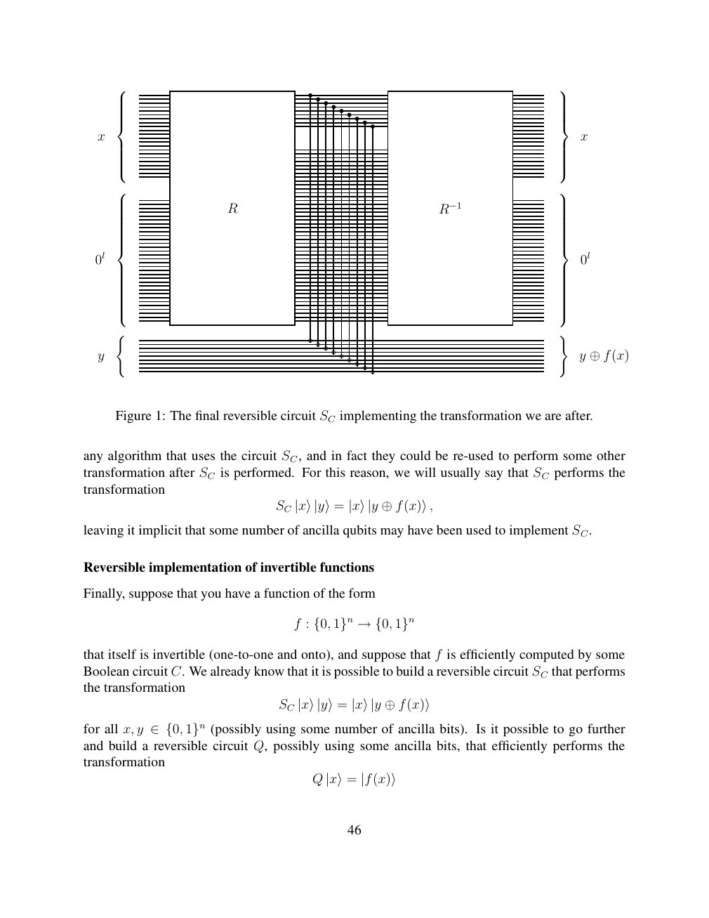
Show extracted searchable text (mathematical glyphs may differ)
x x
R R−1
0l 0l
( )
y y ⊕f(x)
Figure 1: The final reversible circuit SC implementing the transformation we are after.
any algorithm that uses the circuit SC, and in fact they could be re-used to perform some other
transformation after SC is performed. For this reason, we will usually say that SC performs the
transformation
SC |x⟩|y⟩= |x⟩|y ⊕f(x)⟩,
leaving it implicit that some number of ancilla qubits may have been used to implement SC.
Reversible implementation of invertible functions
Finally, suppose that you have a function of the form
f : {0, 1}n →{0, 1}n
that itself is invertible (one-to-one and onto), and suppose that f is efficiently computed by some
Boolean circuit C. We already know that it is possible to build a reversible circuit SC that performs
the transformation
SC |x⟩|y⟩= |x⟩|y ⊕f(x)⟩
for all x, y (possibly using some number of ancilla bits). Is it possible to go further ∈{0, 1}nand build a reversible circuit Q, possibly using some ancilla bits, that efficiently performs the
transformation
Q |x⟩= |f(x)⟩
46
Source page 47
Direct link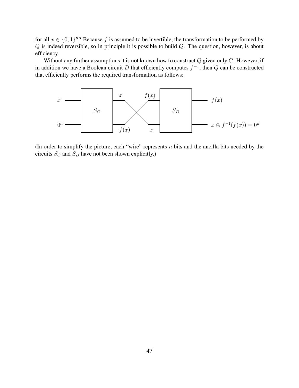
Show extracted searchable text (mathematical glyphs may differ)
for all x Because f is assumed to be invertible, the transformation to be performed by ∈{0, 1}n?Q is indeed reversible, so in principle it is possible to build Q. The question, however, is about
efficiency.
Without any further assumptions it is not known how to construct Q given only C. However, if
in addition we have a Boolean circuit D that efficiently computes f −1, then Q can be constructed
that efficiently performs the required transformation as follows:
x f(x)
x f(x)
SC SD
0n x ⊕f −1(f(x)) = 0n f(x) x
(In order to simplify the picture, each “wire” represents n bits and the ancilla bits needed by the
circuits SC and SD have not been shown explicitly.)
47
⊗ Circuit walkthrough: entanglement and measurement
The Hadamard gate prepares (|0⟩ + |1⟩)/√2 on the first qubit. The controlled-NOT then creates the Bell state (|00⟩ + |11⟩)/√2. Measuring both qubits in the computational basis produces correlated 00 and 11 outcomes, each with ideal probability 1/2. This example illustrates a circuit building block; it is not a complete implementation of the surrounding algorithm.
Show runnable Qiskit example
from qiskit import QuantumCircuit
from qiskit_aer import AerSimulator

qc = QuantumCircuit(2, 2)
qc.h(0)             # Superpose the first qubit
qc.cx(0, 1)         # Entangle both qubits
qc.measure([0, 1], [0, 1])
print(qc.draw(output="text"))
result = AerSimulator().run(qc, shots=1024).result()
print(result.get_counts())  # Approximately 00 and 11
Install qiskit and qiskit-aer locally to execute this code. The diagram is a static circuit illustration, not a browser-based simulator.