Math fidelity: The original PDF page is displayed as a high-resolution image so that equations, bra–ket notation, matrix layouts and circuit diagrams remain exactly as in the source. The expandable text layer is for searching and may not reproduce every mathematical glyph.
Source page 66
Direct link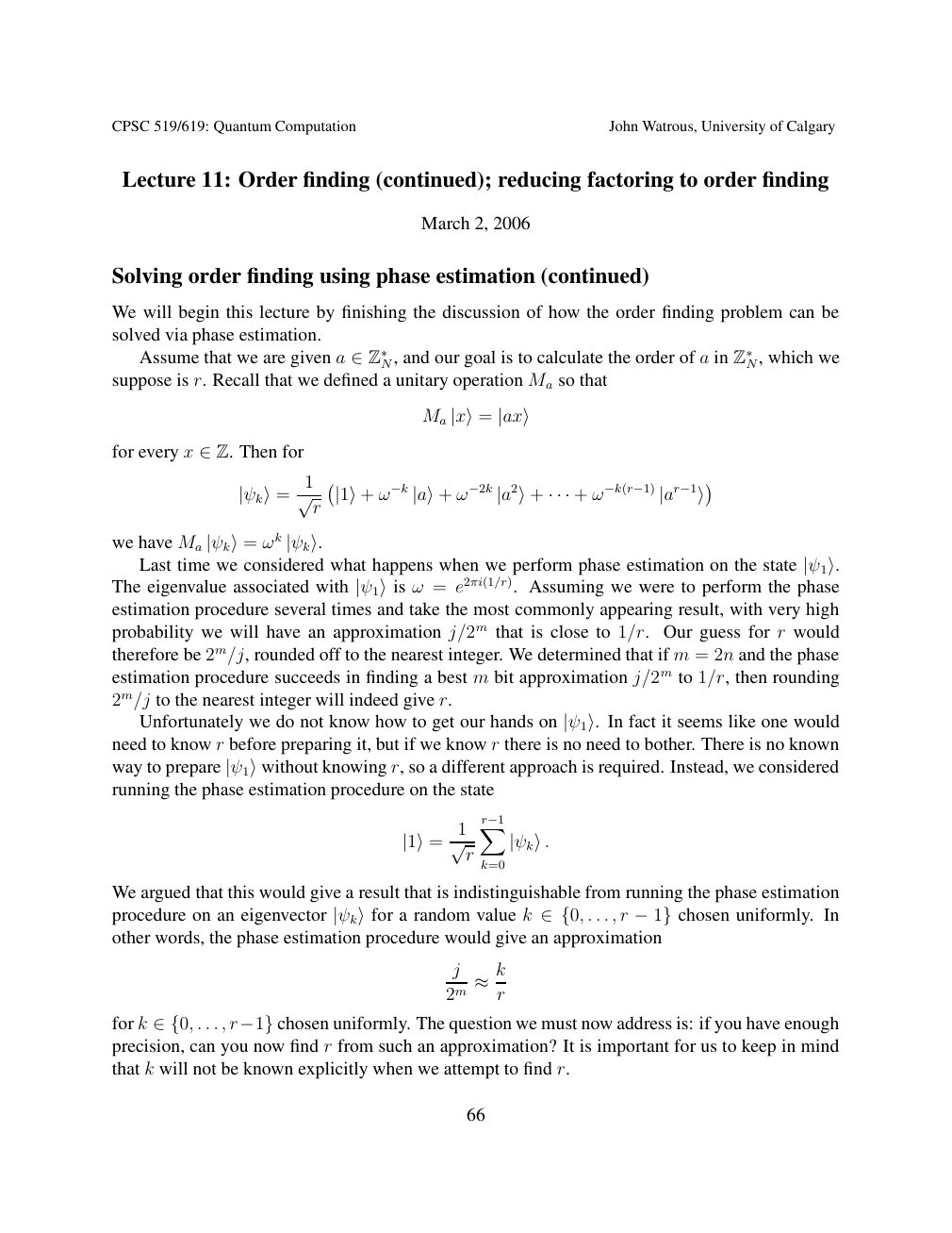
Show extracted searchable text (mathematical glyphs may differ)
CPSC 519/619: Quantum Computation John Watrous, University of Calgary
Lecture 11: Order finding (continued); reducing factoring to order finding
March 2, 2006
Solving order finding using phase estimation (continued)
We will begin this lecture by finishing the discussion of how the order finding problem can be
solved via phase estimation.
a in Z∗N, which we Assume that we are given a ∈Z∗N, and our goal is to calculate the order ofsuppose is r. Recall that we defined a unitary operation Ma so that
Ma |x⟩= |ax⟩
for every x ∈Z. Then for
1
|ψk⟩= √r |1⟩+ ω−k |a⟩+ ω−2k |a2⟩+ · · · + ω−k(r−1) |ar−1⟩
we have Ma ωk |ψk⟩= |ψk⟩.
Last time we considered what happens when we perform phase estimation on the state |ψ1⟩. ω = e2πi(1/r). Assuming we were to perform the phaseThe eigenvalue associated with |ψ1⟩isestimation procedure several times and take the most commonly appearing result, with very high
probability we will have an approximation j/2m that is close to 1/r. Our guess for r would
therefore be 2m/j, rounded off to the nearest integer. We determined that if m = 2n and the phase
estimation procedure succeeds in finding a best m bit approximation j/2m to 1/r, then rounding
2m/j to the nearest integer will indeed give r.
Unfortunately we do not know how to get our hands on |ψ1⟩. In fact it seems like one wouldneed to know r before preparing it, but if we know r there is no need to bother. There is no known
way to prepare |ψ1⟩without knowing r, so a different approach is required. Instead, we consideredrunning the phase estimation procedure on the state
Xr−1 1
|1⟩= √r |ψk⟩.
k=0
We argued that this would give a result that is indistinguishable from running the phase estimation
chosen uniformly. Inprocedure on an eigenvector |ψk⟩for a random value k ∈{0, . . . , r −1}other words, the phase estimation procedure would give an approximation
j
2m ≈kr
for k . . . , chosen uniformly. The question we must now address is: if you have enough ∈{0, r−1}precision, can you now find r from such an approximation? It is important for us to keep in mind
that k will not be known explicitly when we attempt to find r.
66
Source page 67
Direct link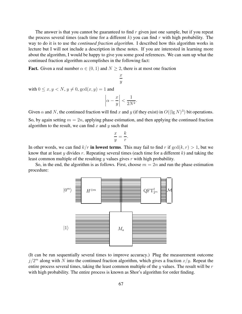
Show extracted searchable text (mathematical glyphs may differ)
The answer is that you cannot be guaranteed to find r given just one sample, but if you repeat
the process several times (each time for a different k) you can find r with high probability. The
way to do it is to use the continued fraction algorithm. I described how this algorithm works in
lecture but I will not include a description in these notes. If you are interested in learning more
about the algorithm, I would be happy to give you some good references. We can sum up what the
continued fraction algorithm accomplishes in the following fact:
Fact. Given a real number α 1) and N there is at most one fraction ∈(0, ≥2,
x
y
with 0 y < N, y 0, gcd(x, y) = 1 and ≤x, ̸=
1
α < . 2 −xy 2N
Given α and N, the continued fraction will find x and y (if they exist) in O((lg N)3) bit operations.
So, by again setting m = 2n, applying phase estimation, and then applying the continued fraction
algorithm to the result, we can find x and y such that
x k
= .
y r
In other words, we can find k/r in lowest terms. This may fail to find r if gcd(k, r) > 1, but we
know that at least y divides r. Repeating several times (each time for a different k) and taking the
least common multiple of the resulting y values gives r with high probability.
So, in the end, the algorithm is as follows. First, choose m = 2n and run the phase estimation
procedure:
2m M |0m⟩ H⊗m QFT†
|1⟩ Ma
(It can be run sequentially several times to improve accuracy.) Plug the measurement outcome
j/2m along with N into the continued fraction algorithm, which gives a fraction x/y. Repeat the
entire process several times, taking the least common multiple of the y values. The result will be r
with high probability. The entire process is known as Shor’s algorithm for order finding.
67
Source page 68
Direct link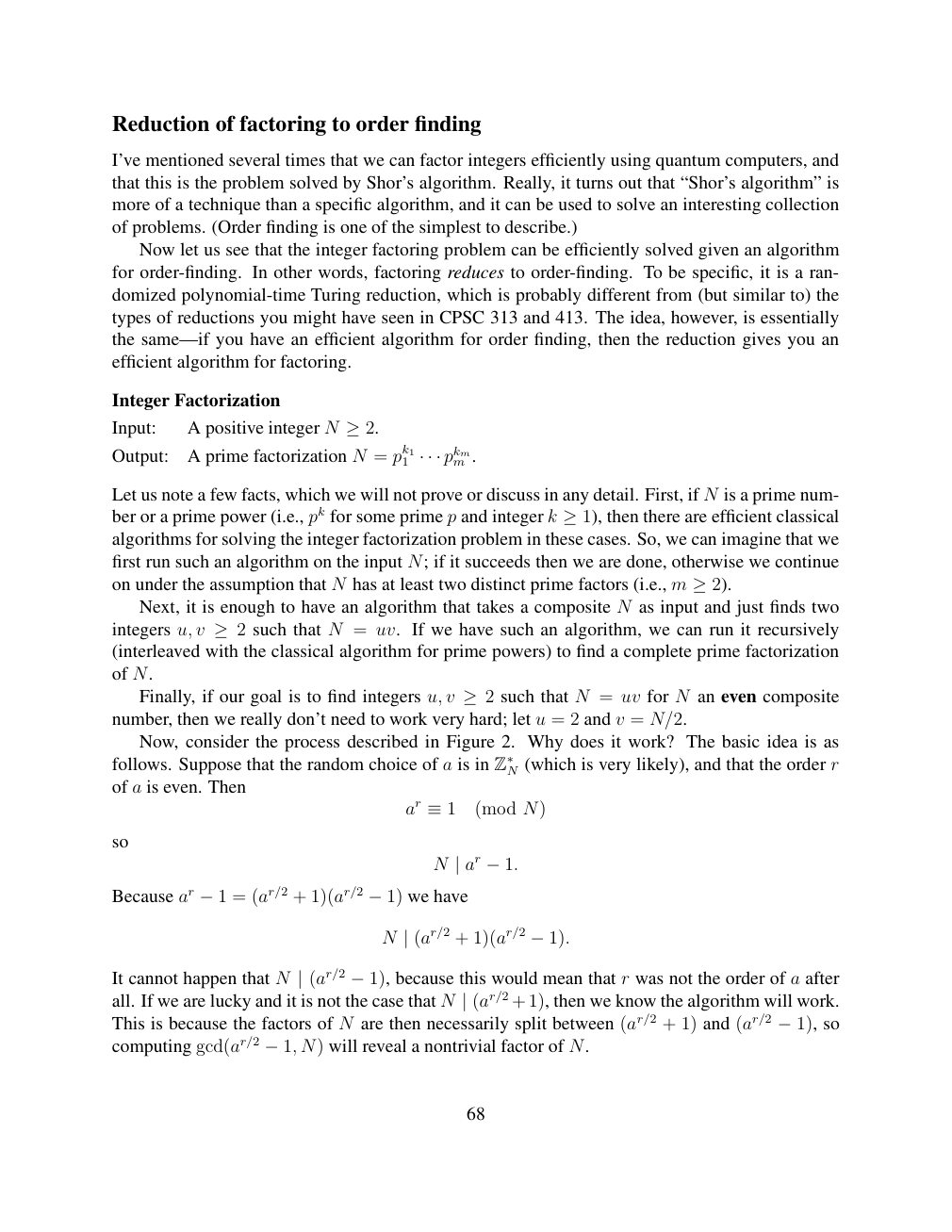
Show extracted searchable text (mathematical glyphs may differ)
Reduction of factoring to order finding
I’ve mentioned several times that we can factor integers efficiently using quantum computers, and
that this is the problem solved by Shor’s algorithm. Really, it turns out that “Shor’s algorithm” is
more of a technique than a specific algorithm, and it can be used to solve an interesting collection
of problems. (Order finding is one of the simplest to describe.)
Now let us see that the integer factoring problem can be efficiently solved given an algorithm
for order-finding. In other words, factoring reduces to order-finding. To be specific, it is a ran-
domized polynomial-time Turing reduction, which is probably different from (but similar to) the
types of reductions you might have seen in CPSC 313 and 413. The idea, however, is essentially
the same—if you have an efficient algorithm for order finding, then the reduction gives you an
efficient algorithm for factoring.
Integer Factorization
Input: A positive integer N ≥2.
Output: A prime factorization N = pk11 pkmm . · · ·
Let us note a few facts, which we will not prove or discuss in any detail. First, if N is a prime num-
ber or a prime power (i.e., pk for some prime p and integer k ≥1), then there are efficient classicalalgorithms for solving the integer factorization problem in these cases. So, we can imagine that we
first run such an algorithm on the input N; if it succeeds then we are done, otherwise we continue
on under the assumption that N has at least two distinct prime factors (i.e., m ≥2). Next, it is enough to have an algorithm that takes a composite N as input and just finds two
integers u, v such that N = uv. If we have such an algorithm, we can run it recursively ≥2(interleaved with the classical algorithm for prime powers) to find a complete prime factorization
of N.
Finally, if our goal is to find integers u, v such that N = uv for N an even composite ≥2number, then we really don’t need to work very hard; let u = 2 and v = N/2.
Now, consider the process described in Figure 2. Why does it work? The basic idea is as
follows. Suppose that the random choice of a is in Z∗N (which is very likely), and that the order r
of a is even. Then
ar ≡1 (mod N)
so
N | ar −1.
Because ar = (ar/2 + 1)(ar/2 we have −1 −1)
N | (ar/2 + 1)(ar/2 −1).
It cannot happen that N (ar/2 because this would mean that r was not the order of a after | −1),all. If we are lucky and it is not the case that N (ar/2 +1), then we know the algorithm will work. |
This is because the factors of N are then necessarily split between (ar/2 + 1) and (ar/2 −1), socomputing gcd(ar/2 N) will reveal a nontrivial factor of N. −1,
68
Source page 69
Direct link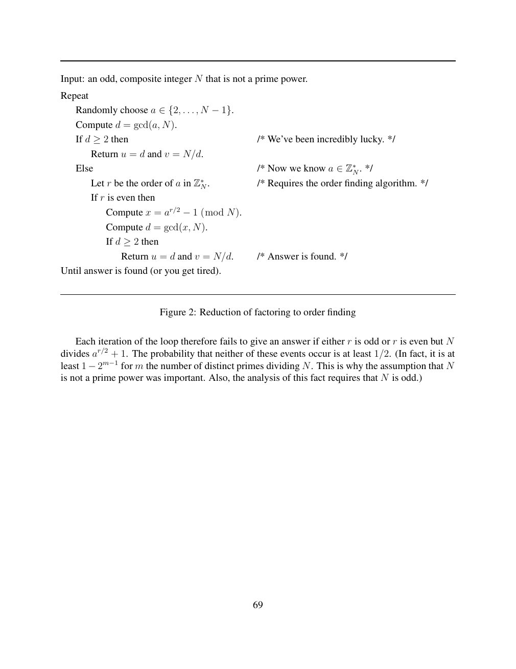
Show extracted searchable text (mathematical glyphs may differ)
Input: an odd, composite integer N that is not a prime power.
Repeat
Randomly choose a . . . , N ∈{2, −1}.
Compute d = gcd(a, N).
If d then /* We’ve been incredibly lucky. */ ≥2
Return u = d and v = N/d.
Else /* Now we know a ∈Z∗N. */
Let r be the order of a in Z∗N. /* Requires the order finding algorithm. */
If r is even then
Compute x = ar/2 (mod N). −1
Compute d = gcd(x, N).
If d then ≥2
Return u = d and v = N/d. /* Answer is found. */
Until answer is found (or you get tired).
Figure 2: Reduction of factoring to order finding
Each iteration of the loop therefore fails to give an answer if either r is odd or r is even but N
divides ar/2 + 1. The probability that neither of these events occur is at least 1/2. (In fact, it is at
m the number of distinct primes dividing N. This is why the assumption that Nleast 1 −2m−1 foris not a prime power was important. Also, the analysis of this fact requires that N is odd.)
69
⊗ Circuit walkthrough: entanglement and measurement
The Hadamard gate prepares (|0⟩ + |1⟩)/√2 on the first qubit. The controlled-NOT then creates the Bell state (|00⟩ + |11⟩)/√2. Measuring both qubits in the computational basis produces correlated 00 and 11 outcomes, each with ideal probability 1/2. This example illustrates a circuit building block; it is not a complete implementation of the surrounding algorithm.
Show runnable Qiskit example
from qiskit import QuantumCircuit
from qiskit_aer import AerSimulator

qc = QuantumCircuit(2, 2)
qc.h(0)             # Superpose the first qubit
qc.cx(0, 1)         # Entangle both qubits
qc.measure([0, 1], [0, 1])
print(qc.draw(output="text"))
result = AerSimulator().run(qc, shots=1024).result()
print(result.get_counts())  # Approximately 00 and 11
Install qiskit and qiskit-aer locally to execute this code. The diagram is a static circuit illustration, not a browser-based simulator.