Math fidelity: The original PDF page is displayed as a high-resolution image so that equations, bra–ket notation, matrix layouts and circuit diagrams remain exactly as in the source. The expandable text layer is for searching and may not reproduce every mathematical glyph.
Source page 76
Direct link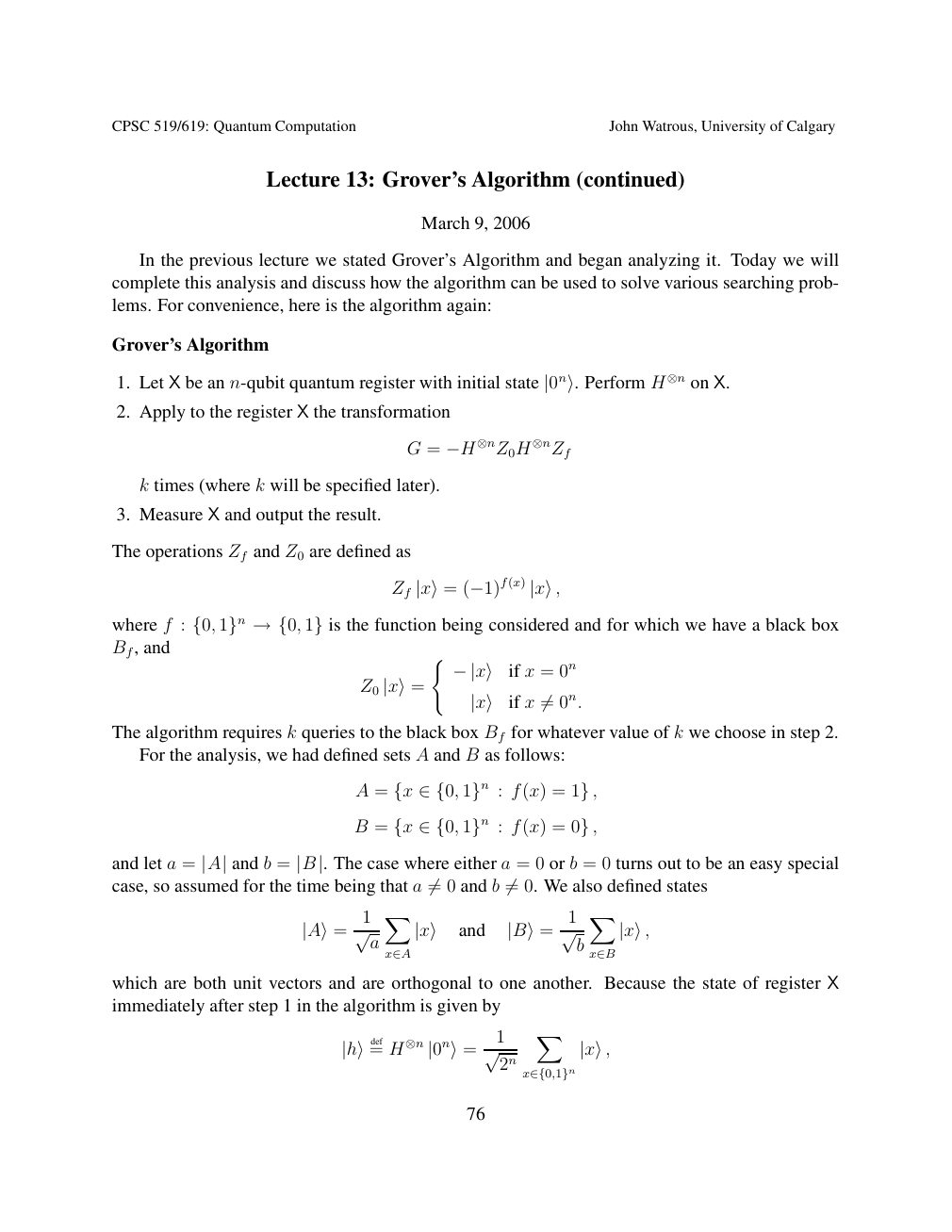
Show extracted searchable text (mathematical glyphs may differ)
CPSC 519/619: Quantum Computation John Watrous, University of Calgary
Lecture 13: Grover’s Algorithm (continued)
March 9, 2006
In the previous lecture we stated Grover’s Algorithm and began analyzing it. Today we will
complete this analysis and discuss how the algorithm can be used to solve various searching prob-
lems. For convenience, here is the algorithm again:
Grover’s Algorithm
1. Let X be an n-qubit quantum register with initial state |0n⟩. Perform H⊗n on X.
2. Apply to the register X the transformation
G = −H⊗nZ0H⊗nZf
k times (where k will be specified later).
3. Measure X and output the result.
The operations Zf and Z0 are defined as
Zf |x⟩= (−1)f(x) |x⟩,
where f : is the function being considered and for which we have a black box {0, 1}n →{0, 1}Bf, and (
if x = 0n Z0 −|x⟩ |x⟩= if x 0n. |x⟩ ̸=
The algorithm requires k queries to the black box Bf for whatever value of k we choose in step 2.
For the analysis, we had defined sets A and B as follows:
A = {x ∈{0, 1}n : f(x) = 1} ,
B = {x ∈{0, 1}n : f(x) = 0} ,
and let a = and b = The case where either a = 0 or b = 0 turns out to be an easy special |A| |B|.case, so assumed for the time being that a 0 and b 0. We also defined states ̸= ̸=
X X 1 1
and |A⟩= √a |x⟩ |B⟩= √ b |x⟩,
x∈A x∈B
which are both unit vectors and are orthogonal to one another. Because the state of register X
immediately after step 1 in the algorithm is given by
X 1 def= H⊗n |h⟩ |0n⟩= √ 2n |x⟩,
x∈{0,1}n
76
Source page 77
Direct link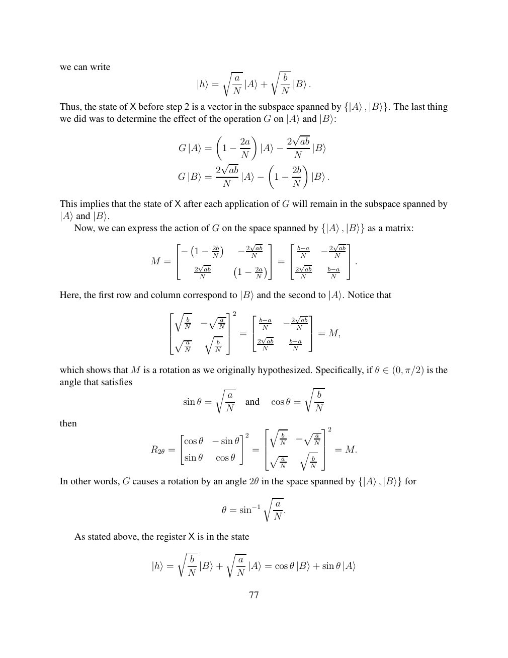
Show extracted searchable text (mathematical glyphs may differ)
we can write r r
a b
|h⟩= N |A⟩+ N |B⟩.
Thus, the state of X before step 2 is a vector in the subspace spanned by The last thing {|A⟩, |B⟩}.
we did was to determine the effect of the operation G on |A⟩and |B⟩:
√ ab
G |A⟩= 1 −2aN |A⟩−2 N |B⟩
2 √ ab
G |B⟩= N |A⟩− 1 −2bN |B⟩.
This implies that the state of X after each application of G will remain in the subspace spanned by
|A⟩and |B⟩. Now, we can express the action of G on the space spanned by as a matrix: {|A⟩, |B⟩}
√ab √ ab 1 b−a − −2bN −2 N N −2 N M = = . 2 √ab 2 √ab 1 b−a N N N N −2a
Here, the first row and column correspond to |B⟩and the second to |A⟩. Notice that
q 2 b a √ab
N N b−aN N −p −2 q = = M, p √ab a b 2 b−a
N N N N
which shows that M is a rotation as we originally hypothesized. Specifically, if θ π/2) is the ∈(0,angle that satisfies r r
a b
sin θ = and cos θ =
N N
then q 2
" #2 b a
cos θ θ N N −p q = M. R2θ = −sin = p sin θ cos θ a b
N N
In other words, G causes a rotation by an angle 2θ in the space spanned by for {|A⟩, |B⟩}
r
a
θ = sin−1 .
N
As stated above, the register X is in the state
r r
b a
|h⟩= N |B⟩+ N |A⟩= cos θ |B⟩+ sin θ |A⟩
77
Source page 78
Direct link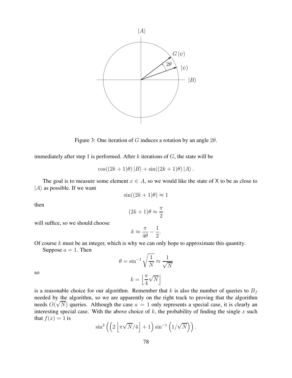
Show extracted searchable text (mathematical glyphs may differ)
|A⟩
G |ψ⟩
2θ
|ψ⟩
|B⟩
Figure 3: One iteration of G induces a rotation by an angle 2θ.
immediately after step 1 is performed. After k iterations of G, the state will be
cos((2k + 1)θ) |B⟩+ sin((2k + 1)θ) |A⟩.
The goal is to measure some element x ∈A, so we would like the state of X to be as close to
|A⟩as possible. If we want
sin((2k + 1)θ) ≈1
then
(2k + 1)θ ≈π2
will suffice, so we should choose
k ≈π4θ −12.
Of course k must be an integer, which is why we can only hope to approximate this quantity.
Suppose a = 1. Then r
1 1
θ = sin−1 N ≈ √ N
so k jπ k = √ N
4
is a reasonable choice for our algorithm. Remember that k is also the number of queries to Bf
needed by the algorithm, so we are apparently on the right track to proving that the algorithm
needs O( √N) queries. Although the case a = 1 only represents a special case, it is clearly an
interesting special case. With the above choice of k, the probability of finding the single x such
that f(x) = 1 is j k
sin2 2 π √ N/4 + 1 sin−1 1/ √N .
78
Source page 79
Direct link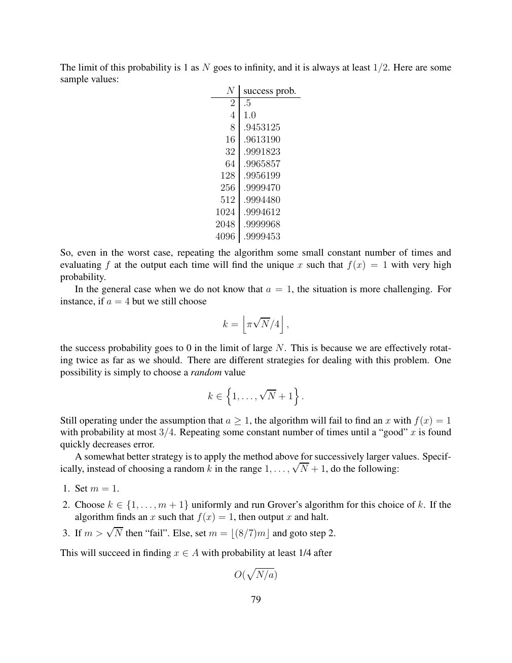
Show extracted searchable text (mathematical glyphs may differ)
The limit of this probability is 1 as N goes to infinity, and it is always at least 1/2. Here are some
sample values:
N success prob.
2 .5
4 1.0
8 .9453125
16 .9613190
32 .9991823
64 .9965857
128 .9956199
256 .9999470
512 .9994480
1024 .9994612
2048 .9999968
4096 .9999453
So, even in the worst case, repeating the algorithm some small constant number of times and
evaluating f at the output each time will find the unique x such that f(x) = 1 with very high
probability.
In the general case when we do not know that a = 1, the situation is more challenging. For
instance, if a = 4 but we still choose
j k
k = π √ N/4 ,
the success probability goes to 0 in the limit of large N. This is because we are effectively rotat-
ing twice as far as we should. There are different strategies for dealing with this problem. One
possibility is simply to choose a random value
n o
k 1, . . . , √N + 1 . ∈
x with f(x) = 1Still operating under the assumption that a ≥1, the algorithm will fail to find anwith probability at most 3/4. Repeating some constant number of times until a “good” x is found
quickly decreases error.
A somewhat better strategy is to apply the method above for successively larger values. Specif-
ically, instead of choosing a random k in the range 1, . . . , √N + 1, do the following:
1. Set m = 1.
2. Choose k . . . , m + uniformly and run Grover’s algorithm for this choice of k. If the ∈{1, 1} algorithm finds an x such that f(x) = 1, then output x and halt.
3. If m > √ N then “fail”. Else, set m = goto step 2. ⌊(8/7)m⌋and
This will succeed in finding x with probability at least 1/4 after ∈A p
O( N/a)
79
Source page 80
Direct link
Show extracted searchable text (mathematical glyphs may differ)
queries. By repeating step 2 a constant number of times during each iteration of the loop, the error
decreases exponentially. (The number 8/7 just happens to be a number that works for the analysis,
which we will not discuss. The point is that m increases exponentially, but not too fast to cause the
algorithm to fail.)
Finally, we still need to deal with the special cases where a = 0 or b = 0. Obviously if a = 0,
the output x of the algorithm will never satisfy f(x) = 1 because there are no such values of x.
It is easy to check directly that Grover’s Algorithm will output a choice of x that is ∈{0, 1}nuniformly distributed in this case. Supposing that we do not know a, if we run Grover’s Algorithm
as described above and always measure a value of x for which f(x) = 0, we can reasonably
conclude with high confidence that a = 0.
It is also the case when b = 0 that Grover’s Algorithm will output a uniformly distributed
choice of x. Of course in this case f(x) = 1 for all x, so the problem is trivially solved.
This represents the end of our discussion of Grover’s algorithm, and of quantum algorithms
in general. The next topics coming up in the course are quantum error correction and quantum
cryptography, with a short discussion of a more general mathematical description of quantum
information than the one we have been using coming first.
80
⊗ Circuit walkthrough: entanglement and measurement
The Hadamard gate prepares (|0⟩ + |1⟩)/√2 on the first qubit. The controlled-NOT then creates the Bell state (|00⟩ + |11⟩)/√2. Measuring both qubits in the computational basis produces correlated 00 and 11 outcomes, each with ideal probability 1/2. This example illustrates a circuit building block; it is not a complete implementation of the surrounding algorithm.
Show runnable Qiskit example
from qiskit import QuantumCircuit
from qiskit_aer import AerSimulator

qc = QuantumCircuit(2, 2)
qc.h(0)             # Superpose the first qubit
qc.cx(0, 1)         # Entangle both qubits
qc.measure([0, 1], [0, 1])
print(qc.draw(output="text"))
result = AerSimulator().run(qc, shots=1024).result()
print(result.get_counts())  # Approximately 00 and 11
Install qiskit and qiskit-aer locally to execute this code. The diagram is a static circuit illustration, not a browser-based simulator.