Math fidelity: The original PDF page is displayed as a high-resolution image so that equations, bra–ket notation, matrix layouts and circuit diagrams remain exactly as in the source. The expandable text layer is for searching and may not reproduce every mathematical glyph.
Source page 81
Direct link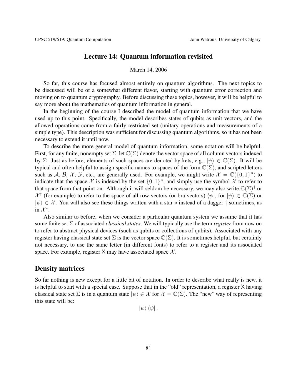
Show extracted searchable text (mathematical glyphs may differ)
CPSC 519/619: Quantum Computation John Watrous, University of Calgary
Lecture 14: Quantum information revisited
March 14, 2006
So far, this course has focused almost entirely on quantum algorithms. The next topics to
be discussed will be of a somewhat different flavor, starting with quantum error correction and
moving on to quantum cryptography. Before discussing these topics, however, it will be helpful to
say more about the mathematics of quantum information in general.
In the beginning of the course I described the model of quantum information that we have
used up to this point. Specifically, the model describes states of qubits as unit vectors, and the
allowed operations come from a fairly restricted set (unitary operations and measurements of a
simple type). This description was sufficient for discussing quantum algorithms, so it has not been
necessary to extend it until now.
To describe the more general model of quantum information, some notation will be helpful.
First, for any finite, nonempty set Σ, let C(Σ) denote the vector space of all column vectors indexed
by Σ. Just as before, elements of such spaces are denoted by kets, e.g., |ψ⟩∈C(Σ). It will betypical and often helpful to assign specific names to spaces of the form C(Σ), and scripted letters
such as A, B, X , Y, etc., are generally used. For example, we might write X = C({0, 1}n) toindicate that the space is indexed by the set and simply use the symbol to refer to X {0, 1}n, Xthat space from that point on. Although it will seldom be necessary, we may also write C(Σ)† or
† (for example) to refer to the space of all row vectors (or bra vectors) for orX ⟨ψ|, |ψ⟩∈C(Σ) . You will also see these things written with a star of a dagger sometimes, as|ψ⟩∈X ∗instead †in ∗. X Also similar to before, when we consider a particular quantum system we assume that it has
some finite set Σ of associated classical states. We will typically use the term register from now on
to refer to abstract physical devices (such as qubits or collections of qubits). Associated with any
register having classical state set Σ is the vector space C(Σ). It is sometimes helpful, but certainly
not necessary, to use the same letter (in different fonts) to refer to a register and its associated
space. For example, register X may have associated space . X
Density matrices
So far nothing is new except for a little bit of notation. In order to describe what really is new, it
is helpful to start with a special case. Suppose that in the “old” representation, a register X having
classical state set Σ is in a quantum state for = C(Σ). The “new” way of representing |ψ⟩∈X Xthis state will be:
|ψ⟩⟨ψ| .
81
Source page 82
Direct link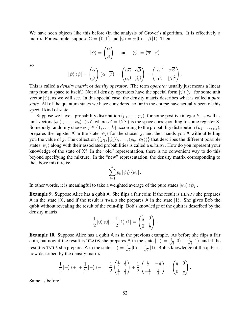
Show extracted searchable text (mathematical glyphs may differ)
We have seen objects like this before (in the analysis of Grover’s algorithm. It is effectively a
matrix. For example, suppose Σ = and α β Then {0, 1} |ψ⟩= |0⟩+ |1⟩. !
α
and = α β |ψ⟩= β ⟨ψ|
so ! ! !
α αα αβ = |α|2 αβ . = α β = |ψ⟩⟨ψ| β αβ ββ αβ |β|2
This is called a density matrix or density operator. (The term operator usually just means a linear
map from a space to itself.) Not all density operators have the special form for some unit |ψ⟩⟨ψ|
vector |ψ⟩, as we will see. In this special case, the density matrix describes what is called a purestate. All of the quantum states we have considered so far in the course have actually been of this
special kind of state.
Suppose we have a probability distribution (p1, . . . , pk), for some positive integer k, as well as
unit vectors . . . , , where = C(Σ) is the space corresponding to some register X. |ψ1⟩, |ψk⟩∈X XSomebody randomly chooses j . . . , according to the probability distribution (p1, . . . , pk), ∈{1, k}
prepares the register X in the state |ψj⟩for the chosen j, and then hands you X without tellingyou the value of j. The collection . . . , (pk, that describes the different possible {(p1, |ψ1⟩), |ψk⟩)}
states |ψj⟩along with their associated probabilities is called a mixture. How do you represent yourknowledge of the state of X? In the “old” representation, there is no convenient way to do this
beyond specifying the mixture. In the “new” representation, the density matrix corresponding to
the above mixture is:
Xk
pk |ψj⟩⟨ψj| .
j=1
In other words, it is meaningful to take a weighted average of the pure states |ψj⟩⟨ψj|.
Example 9. Suppose Alice has a qubit A. She flips a fair coin: if the result is HEADS she prepares
A in the state |0⟩, and if the result is TAILS she prepares A in the state |1⟩. She gives Bob thequbit without revealing the result of the coin-flip. Bob’s knowledge of the qubit is described by the
density matrix !
1 0 1 1 2
+ = .
1 2 |0⟩⟨0| 2 |1⟩⟨1| 0 2
Example 10. Suppose Alice has a qubit A as in the previous example. As before she flips a fair
coin, but now if the result is HEADS she prepares A in the state √12 √12 and if the |+⟩= |0⟩+ |1⟩,
Bob’s knowledge of the qubit isresult is TAILS she prepares A in the state √12 √12 |−⟩= |0⟩− |1⟩.now described by the density matrix
! ! !
1 1 1 0 1 1 1 2 2 1 2 2 2 1 −1 . + = + = 2 |+⟩⟨+| 2 |−⟩⟨−| 2 1 1 2 1 0 1 2 2 2 2 2 −1
Same as before!
82
Source page 83
Direct link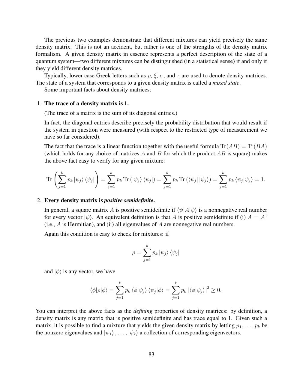
Show extracted searchable text (mathematical glyphs may differ)
The previous two examples demonstrate that different mixtures can yield precisely the same
density matrix. This is not an accident, but rather is one of the strengths of the density matrix
formalism. A given density matrix in essence represents a perfect description of the state of a
quantum system—two different mixtures can be distinguished (in a statistical sense) if and only if
they yield different density matrices.
Typically, lower case Greek letters such as ρ, ξ, σ, and τ are used to denote density matrices.
The state of a system that corresponds to a given density matrix is called a mixed state.
Some important facts about density matrices:
1. The trace of a density matrix is 1.
(The trace of a matrix is the sum of its diagonal entries.)
In fact, the diagonal entries describe precisely the probability distribution that would result if
the system in question were measured (with respect to the restricted type of measurement we
have so far considered).
The fact that the trace is a linear function together with the useful formula Tr(AB) = Tr(BA)
(which holds for any choice of matrices A and B for which the product AB is square) makes
the above fact easy to verify for any given mixture:
!
Xk Xk Xk Xk
Tr pk |ψj⟩⟨ψj| = pk Tr (|ψj⟩⟨ψj|) = pk Tr (⟨ψj| |ψj⟩) = pk ⟨ψj|ψj⟩= 1.
j=1 j=1 j=1 j=1
2. Every density matrix is positive semidefinite.
In general, a square matrix A is positive semidefinite if ⟨ψ|A|ψ⟩is a nonnegative real number A is positive semidefinite if (i) A = A† for every vector |ψ⟩. An equivalent definition is that (i.e., A is Hermitian), and (ii) all eigenvalues of A are nonnegative real numbers.
Again this condition is easy to check for mixtures: if
Xk
ρ = pk |ψj⟩⟨ψj|
j=1
and |φ⟩is any vector, we have
Xk Xk
⟨φ|ρ|φ⟩= pk ⟨φ|ψj⟩⟨ψj|φ⟩= pk |⟨φ|ψj⟩|2 ≥0.
j=1 j=1
You can interpret the above facts as the defining properties of density matrices: by definition, a
density matrix is any matrix that is positive semidefinite and has trace equal to 1. Given such a
matrix, it is possible to find a mixture that yields the given density matrix by letting p1, . . . , pk be
the nonzero eigenvalues and . . . , collection of corresponding eigenvectors. |ψ1⟩, |ψk⟩a
83
Source page 84
Direct link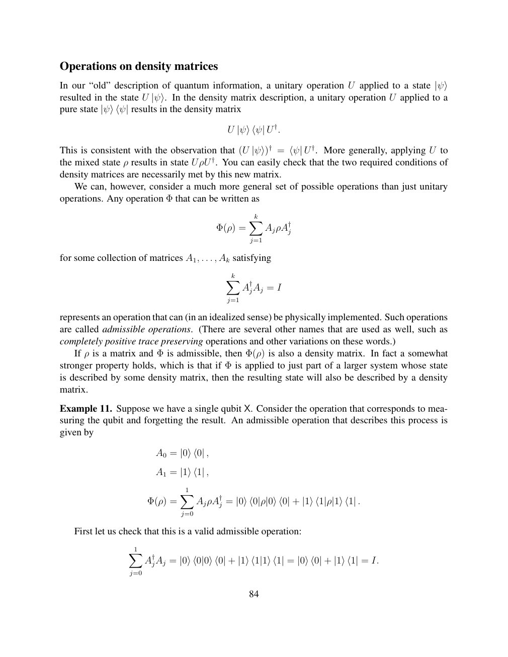
Show extracted searchable text (mathematical glyphs may differ)
Operations on density matrices
In our “old” description of quantum information, a unitary operation U applied to a state |ψ⟩ U applied to aresulted in the state U |ψ⟩. In the density matrix description, a unitary operationpure state results in the density matrix |ψ⟩⟨ψ|
U |ψ⟩⟨ψ| U †.
†. More generally, applying U toThis is consistent with the observation that (U |ψ⟩)† = ⟨ψ| Uthe mixed state ρ results in state UρU †. You can easily check that the two required conditions of
density matrices are necessarily met by this new matrix.
We can, however, consider a much more general set of possible operations than just unitary
operations. Any operation Φ that can be written as
Xk
Φ(ρ) = AjρA†j
j=1
for some collection of matrices A1, . . . , Ak satisfying
Xk
A†jAj = I
j=1
represents an operation that can (in an idealized sense) be physically implemented. Such operations
are called admissible operations. (There are several other names that are used as well, such as
completely positive trace preserving operations and other variations on these words.)
If ρ is a matrix and Φ is admissible, then Φ(ρ) is also a density matrix. In fact a somewhat
stronger property holds, which is that if Φ is applied to just part of a larger system whose state
is described by some density matrix, then the resulting state will also be described by a density
matrix.
Example 11. Suppose we have a single qubit X. Consider the operation that corresponds to mea-
suring the qubit and forgetting the result. An admissible operation that describes this process is
given by
A0 = |0⟩⟨0| ,
A1 = |1⟩⟨1| ,
X1
Φ(ρ) = AjρA†j = |0⟩⟨0|ρ|0⟩⟨0| + |1⟩⟨1|ρ|1⟩⟨1| .
j=0
First let us check that this is a valid admissible operation:
X1
A†jAj = |0⟩⟨0|0⟩⟨0| + |1⟩⟨1|1⟩⟨1| = |0⟩⟨0| + |1⟩⟨1| = I.
j=0
84
Source page 85
Direct link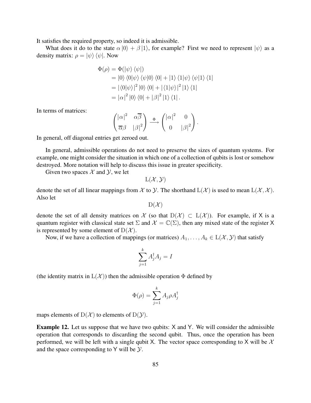
Show extracted searchable text (mathematical glyphs may differ)
It satisfies the required property, so indeed it is admissible.
What does it do to the state α β for example? First we need to represent a |0⟩+ |1⟩, |ψ⟩as
density matrix: ρ = |ψ⟩⟨ψ|. Now
Φ(ρ) = Φ(|ψ⟩⟨ψ|)
= |0⟩⟨0|ψ⟩⟨ψ|0⟩⟨0| + |1⟩⟨1|ψ⟩⟨ψ|1⟩⟨1|
= |⟨0|ψ⟩|2 |0⟩⟨0| + |⟨1|ψ⟩|2 |1⟩⟨1|
= |α|2 |0⟩⟨0| + |β|2 |1⟩⟨1| .
In terms of matrices: ! !
Φ |α|2 αβ |α|2 0 . αβ −→ 0 |β|2 |β|2
In general, off diagonal entries get zeroed out.
In general, admissible operations do not need to preserve the sizes of quantum systems. For
example, one might consider the situation in which one of a collection of qubits is lost or somehow
destroyed. More notation will help to discuss this issue in greater specificity.
Given two spaces and we let X Y,
L(X , Y)
denote the set of all linear mappings from to The shorthand ) is used to mean , ). X Y. L(X L(X XAlso let
D(X )
denote the set of all density matrices on (so that ) )). For example, if X is a X D(X ⊂L(X Xquantum register with classical state set Σ and = C(Σ), then any mixed state of the register Xis represented by some element of ). D(X Now, if we have a collection of mappings (or matrices) A1, . . . , Ak , that satisfy ∈L(X Y)
Xk
A†jAj = I
j=1
(the identity matrix in )) then the admissible operation Φ defined by L(X
Xk
Φ(ρ) = AjρA†j
j=1
maps elements of ) to elements of D(X D(Y).
Example 12. Let us suppose that we have two qubits: X and Y. We will consider the admissible
operation that corresponds to discarding the second qubit. Thus, once the operation has been
performed, we will be left with a single qubit X. The vector space corresponding to X will be Y Xand the space corresponding to will be Y.
85
Source page 86
Direct link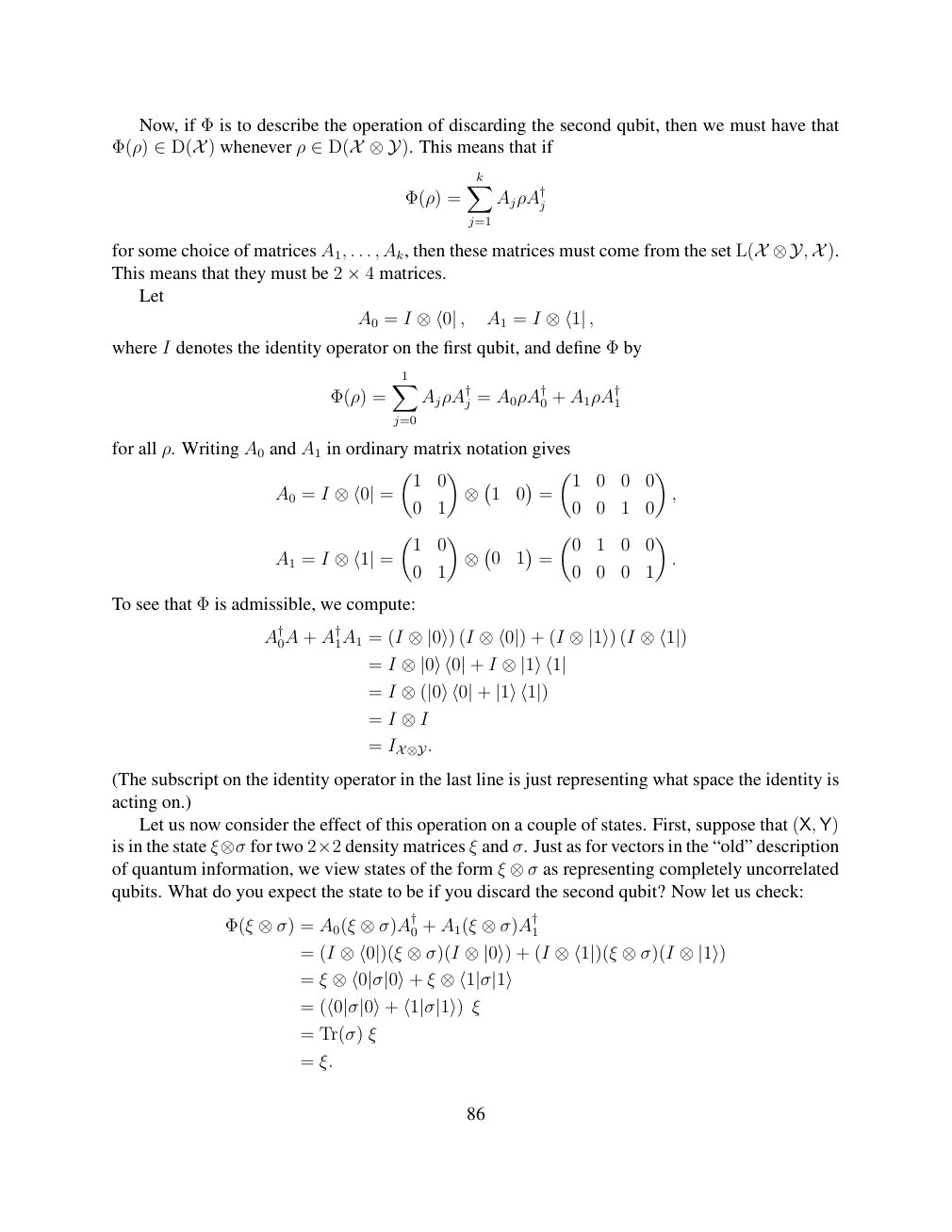
Show extracted searchable text (mathematical glyphs may differ)
Now, if Φ is to describe the operation of discarding the second qubit, then we must have that
Φ(ρ) ) whenever ρ This means that if ∈D(X ∈D(X ⊗Y).
Xk
Φ(ρ) = AjρA†j
j=1
for some choice of matrices A1, . . . , Ak, then these matrices must come from the set ). L(X ⊗Y, XThis means that they must be 2 4 matrices. × Let
A0 = I ⊗⟨0| , A1 = I ⊗⟨1| ,
where I denotes the identity operator on the first qubit, and define Φ by
X1
Φ(ρ) = AjρA†j = A0ρA†0 + A1ρA†1
j=0
for all ρ. Writing A0 and A1 in ordinary matrix notation gives
1 0 1 0 0 0
A0 = I ⊗⟨0| = 0 1 ⊗ 1 0 = 0 0 1 0 ,
1 0 0 1 0 0
A1 = I ⊗⟨1| = 0 1 ⊗ 0 1 = 0 0 0 1 .
To see that Φ is admissible, we compute:
A†0A + A†1A1 = (I ⊗|0⟩) (I ⊗⟨0|) + (I ⊗|1⟩) (I ⊗⟨1|)
= I ⊗|0⟩⟨0| + I ⊗|1⟩⟨1|
= I ⊗(|0⟩⟨0| + |1⟩⟨1|)
= I ⊗I
= IX ⊗Y.
(The subscript on the identity operator in the last line is just representing what space the identity is
acting on.)
Let us now consider the effect of this operation on a couple of states. First, suppose that (X, Y)
is in the state for two density matrices ξ and σ. Just as for vectors in the “old” description ξ⊗σ 2×2of quantum information, we view states of the form ξ as representing completely uncorrelated ⊗σqubits. What do you expect the state to be if you discard the second qubit? Now let us check:
1 Φ(ξ ⊗σ) = A0(ξ ⊗σ)A† 0 + A1(ξ ⊗σ)A†
= (I ⊗⟨0|)(ξ ⊗σ)(I ⊗|0⟩) + (I ⊗⟨1|)(ξ ⊗σ)(I ⊗|1⟩)
= ξ ⊗⟨0|σ|0⟩+ ξ ⊗⟨1|σ|1⟩
= (⟨0|σ|0⟩+ ⟨1|σ|1⟩) ξ
= Tr(σ) ξ
= ξ.
86
Source page 87
Direct link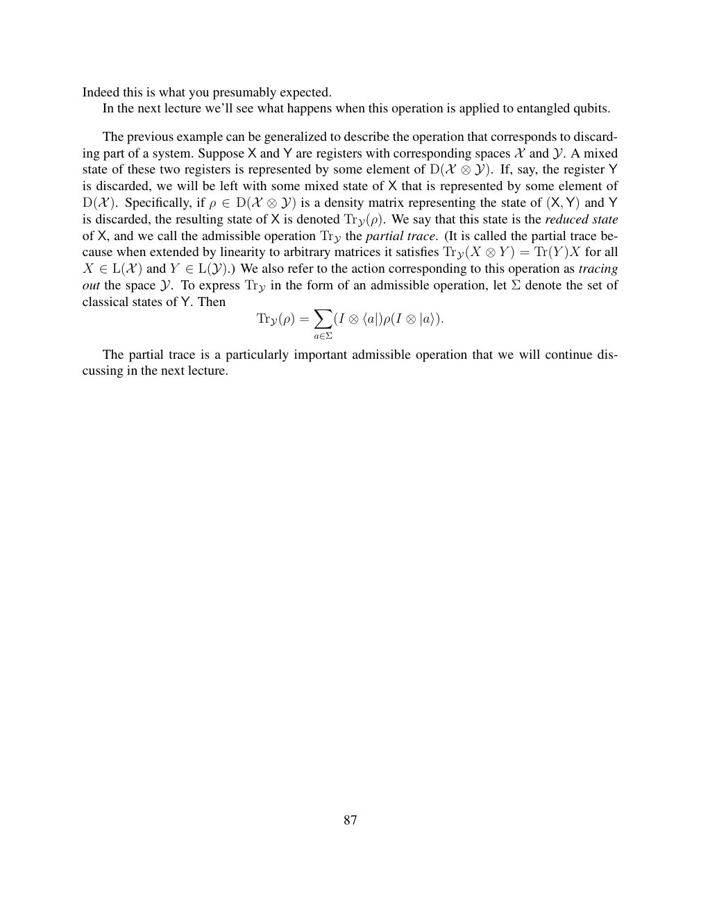
Show extracted searchable text (mathematical glyphs may differ)
Indeed this is what you presumably expected.
In the next lecture we’ll see what happens when this operation is applied to entangled qubits.
The previous example can be generalized to describe the operation that corresponds to discard-
ing part of a system. Suppose X and Y are registers with corresponding spaces and A mixed X Y. Ystate of these two registers is represented by some element of If, say, the register D(X ⊗Y).is discarded, we will be left with some mixed state of X that is represented by some element of
). Specifically, if ρ is a density matrix representing the state of (X, Y) and YD(X ∈D(X ⊗Y)Xis discarded, the resulting state of is denoted TrY(ρ). We say that this state is the reduced state
of X, and we call the admissible operation the partial trace. (It is called the partial trace be- TrY
cause when extended by linearity to arbitrary matrices it satisfies ) = Tr(Y )X for all TrY(X ⊗YX ) and Y We also refer to the action corresponding to this operation as tracing ∈L(X ∈L(Y).)
out the space Y. To express TrY in the form of an admissible operation, let Σ denote the set ofclassical states of Y. Then X
TrY(ρ) = (I ⊗⟨a|)ρ(I ⊗|a⟩).
a∈Σ
The partial trace is a particularly important admissible operation that we will continue dis-
cussing in the next lecture.
87
⊗ Circuit walkthrough: entanglement and measurement
The Hadamard gate prepares (|0⟩ + |1⟩)/√2 on the first qubit. The controlled-NOT then creates the Bell state (|00⟩ + |11⟩)/√2. Measuring both qubits in the computational basis produces correlated 00 and 11 outcomes, each with ideal probability 1/2. This example illustrates a circuit building block; it is not a complete implementation of the surrounding algorithm.
Show runnable Qiskit example
from qiskit import QuantumCircuit
from qiskit_aer import AerSimulator

qc = QuantumCircuit(2, 2)
qc.h(0)             # Superpose the first qubit
qc.cx(0, 1)         # Entangle both qubits
qc.measure([0, 1], [0, 1])
print(qc.draw(output="text"))
result = AerSimulator().run(qc, shots=1024).result()
print(result.get_counts())  # Approximately 00 and 11
Install qiskit and qiskit-aer locally to execute this code. The diagram is a static circuit illustration, not a browser-based simulator.