Math fidelity: The original PDF page is displayed as a high-resolution image so that equations, bra–ket notation, matrix layouts and circuit diagrams remain exactly as in the source. The expandable text layer is for searching and may not reproduce every mathematical glyph.
Source page 70
Direct link
Show extracted searchable text (mathematical glyphs may differ)
CPSC 519/619: Quantum Computation John Watrous, University of Calgary
Lecture 12: Grover’s Algorithm
March 7, 2006
We have completed our study of Shor’s factoring algorithm. The basic technique behind Shor’s
algorithm, which we described in terms of phase estimation, can also be used to solve some other
number-theoretic and group-theoretic problems as well (such as computing discrete logarithms
and calculating orders of abelian groups). This family of problems represents one of the main
reasons why there is such great interest in building quantum computers, as the associated quan-
tum algorithms give an exponential advantage over the best known classical algorithms for these
problems.
We will now study a different quantum algorithmic technique. It does not give as impressive an
advantage over classical algorithms as we have for Shor’s algorithm, but the technique is applicable
to a much broader class of problems. The simplest general problem to which this technique can be
applied is search; and although there are other applications of the technique, this will be the focus
of our investigation. The technique was first considered by Lov Grover, and is known as Grover’s
Algorithm in the context of search.
Unstructured search
We will be returning to the black-box context that was used to describe Deutsch’s algorithm, the
Deutsch-Jozsa algorithm, and Simon’s algorithm. (The fact that Grover’s algorithm works in this
very general context represents one of its strengths, because in general there will not need to be
any promises on the black box.) Suppose that we have a function
f : {0, 1}n →{0, 1}
that is implemented by a reversible transformation Bf in the usual way:
Bf |x⟩|a⟩= |x⟩|a ⊕f(x)⟩
for all x and a The problem of search is simply to find a string x ∈{0, 1}n ∈{0, 1} ∈{0, 1}nsuch that f(x) = 1, or to conclude that no such x exists if f is identically 0).
It is important to note that this searching problem is completely unstructured. There are no
promises on the function f, so it is not possible to use binary search or any other fast searching
method to efficiently solve the problem classically.
What is the best classical algorithm for solving the above search problem? As we have noted
before, it is more complicated than one might initially think to rigorously prove lower bounds
on algorithms. In this particular case it is not too hard, but because our focus is on the quantum
algorithm for the problem we will only discuss informally the issue of classical complexity.
70
Source page 71
Direct link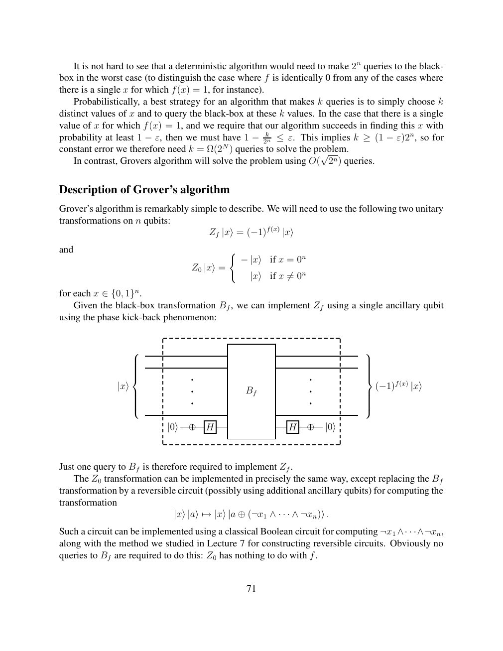
Show extracted searchable text (mathematical glyphs may differ)
It is not hard to see that a deterministic algorithm would need to make 2n queries to the black-
box in the worst case (to distinguish the case where f is identically 0 from any of the cases where
there is a single x for which f(x) = 1, for instance).
Probabilistically, a best strategy for an algorithm that makes k queries is to simply choose k
distinct values of x and to query the black-box at these k values. In the case that there is a single
value of x for which f(x) = 1, and we require that our algorithm succeeds in finding this x with
2n k ≤ε. This implies k ≥(1 −ε)2n, so forprobability at least 1 −ε, then we must have 1 −constant error we therefore need k = Ω(2N) queries to solve the problem.
In contrast, Grovers algorithm will solve the problem using O( √2n) queries.
Description of Grover’s algorithm
Grover’s algorithm is remarkably simple to describe. We will need to use the following two unitary
transformations on n qubits:
Zf |x⟩= (−1)f(x) |x⟩
and (
if x = 0n Z0 −|x⟩ |x⟩= if x 0n |x⟩ ̸=
for each x ∈{0, 1}n. Given the black-box transformation Bf, we can implement Zf using a single ancillary qubit
using the phase kick-back phenomenon:
Bf (−1)f(x) |x⟩ |x⟩
|0⟩ H H |0⟩
Just one query to Bf is therefore required to implement Zf.
The Z0 transformation can be implemented in precisely the same way, except replacing the Bf
transformation by a reversible circuit (possibly using additional ancillary qubits) for computing the
transformation
|x⟩|a⟩7→|x⟩|a ⊕(¬x1 ∧· · · ∧¬xn)⟩.
Such a circuit can be implemented using a classical Boolean circuit for computing ¬x1 ∧· · ·∧¬xn,along with the method we studied in Lecture 7 for constructing reversible circuits. Obviously no
queries to Bf are required to do this: Z0 has nothing to do with f.
71
Source page 72
Direct link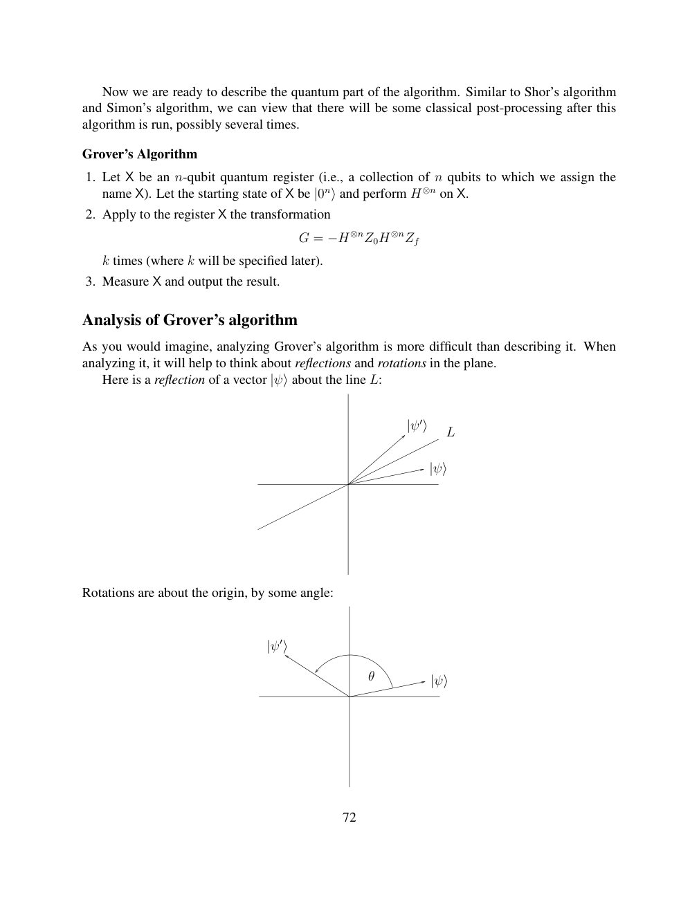
Show extracted searchable text (mathematical glyphs may differ)
Now we are ready to describe the quantum part of the algorithm. Similar to Shor’s algorithm
and Simon’s algorithm, we can view that there will be some classical post-processing after this
algorithm is run, possibly several times.
Grover’s Algorithm
1. Let X be an n-qubit quantum register (i.e., a collection of n qubits to which we assign the
name X). Let the starting state of X be |0n⟩and perform H⊗n on X.
2. Apply to the register X the transformation
G = −H⊗nZ0H⊗nZf
k times (where k will be specified later).
3. Measure X and output the result.
Analysis of Grover’s algorithm
As you would imagine, analyzing Grover’s algorithm is more difficult than describing it. When
analyzing it, it will help to think about reflections and rotations in the plane.
Here is a reflection of a vector |ψ⟩about the line L:
|ψ′⟩ L
|ψ⟩
Rotations are about the origin, by some angle:
|ψ′⟩
θ
|ψ⟩
72
Source page 73
Direct link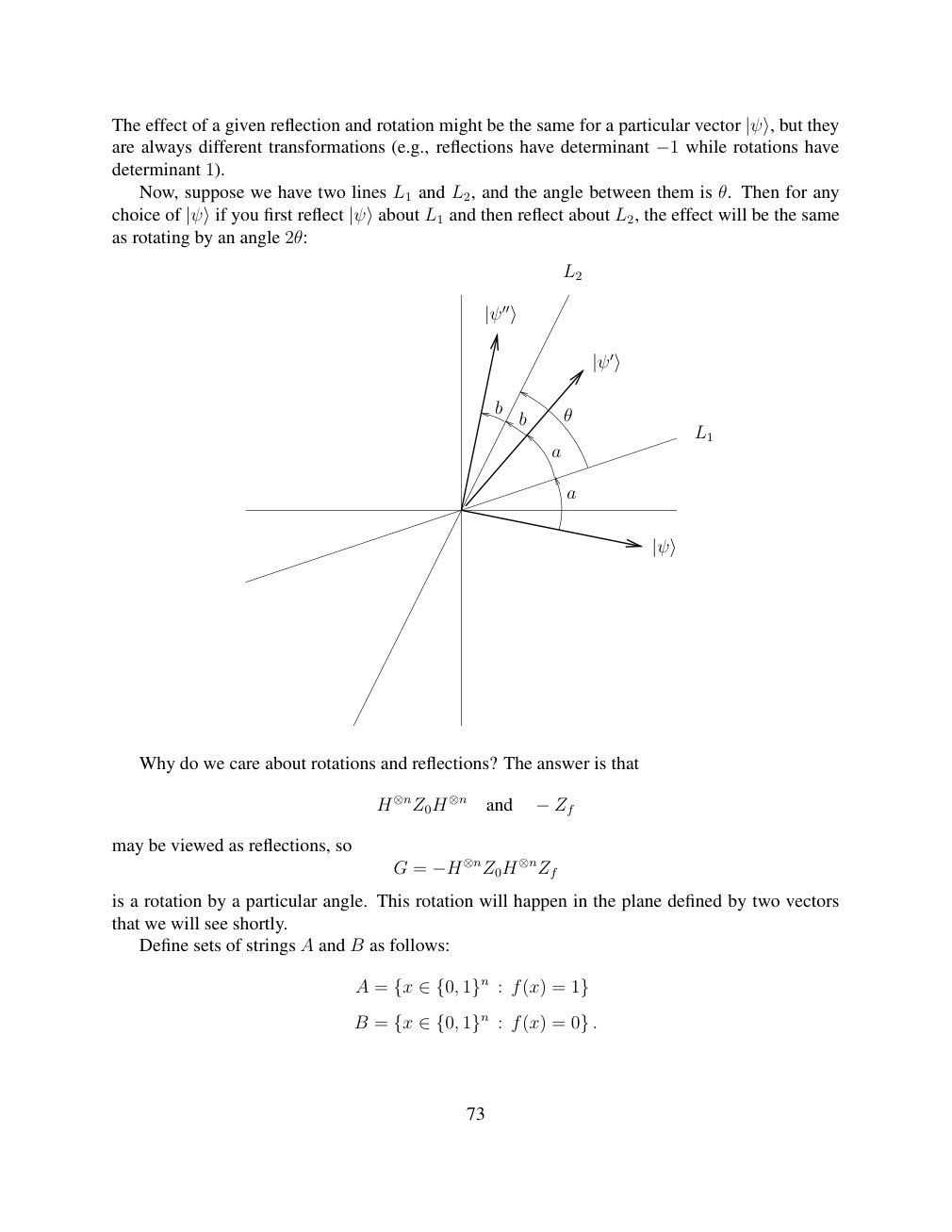
Show extracted searchable text (mathematical glyphs may differ)
The effect of a given reflection and rotation might be the same for a particular vector |ψ⟩, but theyare always different transformations (e.g., reflections have determinant while rotations have −1determinant 1).
Now, suppose we have two lines L1 and L2, and the angle between them is θ. Then for any
L1 and then reflect about L2, the effect will be the samechoice of |ψ⟩if you first reflect |ψ⟩aboutas rotating by an angle 2θ:
L2
|ψ′′⟩
|ψ′⟩
b
b θ
L1
a
a
|ψ⟩
Why do we care about rotations and reflections? The answer is that
H⊗nZ0H⊗n and −Zf
may be viewed as reflections, so
G = −H⊗nZ0H⊗nZf
is a rotation by a particular angle. This rotation will happen in the plane defined by two vectors
that we will see shortly.
Define sets of strings A and B as follows:
A = {x ∈{0, 1}n : f(x) = 1}
B = {x ∈{0, 1}n : f(x) = 0} .
73
Source page 74
Direct link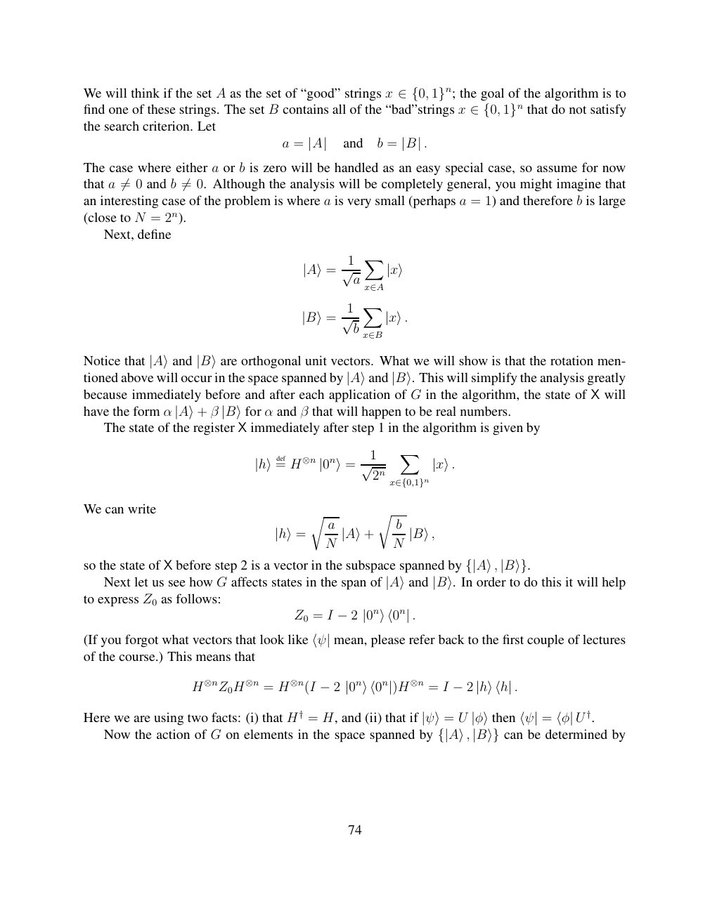
Show extracted searchable text (mathematical glyphs may differ)
We will think if the set A as the set of “good” strings x the goal of the algorithm is to ∈{0, 1}n;find one of these strings. The set B contains all of the “bad”strings x that do not satisfy ∈{0, 1}nthe search criterion. Let
a = and b = . |A| |B|
The case where either a or b is zero will be handled as an easy special case, so assume for now
that a 0 and b 0. Although the analysis will be completely general, you might imagine that ̸= ̸=an interesting case of the problem is where a is very small (perhaps a = 1) and therefore b is large
(close to N = 2n).
Next, define
X 1
|A⟩= √a |x⟩
x∈A
X 1
|B⟩= √ b |x⟩.
x∈B
Notice that |A⟩and |B⟩are orthogonal unit vectors. What we will show is that the rotation men-
tioned above will occur in the space spanned by |A⟩and |B⟩. This will simplify the analysis greatlybecause immediately before and after each application of G in the algorithm, the state of X will
have the form α β α and β that will happen to be real numbers. |A⟩+ |B⟩forX The state of the register immediately after step 1 in the algorithm is given by
X 1 def= H⊗n |h⟩ |0n⟩= √ 2n |x⟩.
x∈{0,1}n
We can write r r
a b
|h⟩= N |A⟩+ N |B⟩,
so the state of X before step 2 is a vector in the subspace spanned by {|A⟩, |B⟩}.
Next let us see how G affects states in the span of |A⟩and |B⟩. In order to do this it will helpto express Z0 as follows:
Z0 = I −2 |0n⟩⟨0n| .
(If you forgot what vectors that look like mean, please refer back to the first couple of lectures ⟨ψ|of the course.) This means that
H⊗nZ0H⊗n = H⊗n(I −2 |0n⟩⟨0n|)H⊗n = I −2 |h⟩⟨h| .
Here we are using two facts: (i) that H† = H, and (ii) that if U = U †. |ψ⟩= |φ⟩then ⟨ψ| ⟨φ| Now the action of G on elements in the space spanned by can be determined by {|A⟩, |B⟩}
74
Source page 75
Direct link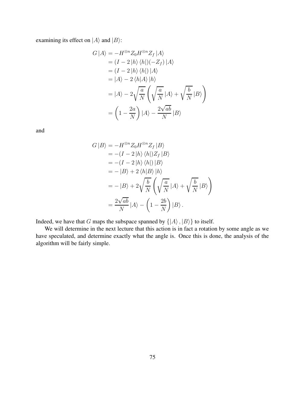
Show extracted searchable text (mathematical glyphs may differ)
examining its effect on |A⟩and |B⟩:
G |A⟩= −H⊗nZ0H⊗nZf |A⟩
= (I −2 |h⟩⟨h|)(−Zf) |A⟩
= (I −2 |h⟩⟨h|) |A⟩
= |A⟩−2 r⟨h|A⟩|h⟩r r !
a a b
= |A⟩−2 N N |A⟩+ N |B⟩
√ ab
= 1 −2aN |A⟩−2 N |B⟩
and
G |B⟩= −H⊗nZ0H⊗nZf |B⟩
= −(I −2 |h⟩⟨h|)Zf |B⟩
= −(I −2 |h⟩⟨h|) |B⟩
= −|B⟩+ 2 r⟨h|B⟩|h⟩r r !
b a b
= −|B⟩+ 2 N N |A⟩+ N |B⟩
2 √ ab
= 1 N |A⟩− −2bN |B⟩.
Indeed, we have that G maps the subspace spanned by to itself. {|A⟩, |B⟩} We will determine in the next lecture that this action is in fact a rotation by some angle as we
have speculated, and determine exactly what the angle is. Once this is done, the analysis of the
algorithm will be fairly simple.
75
⊗ Circuit walkthrough: entanglement and measurement
The Hadamard gate prepares (|0⟩ + |1⟩)/√2 on the first qubit. The controlled-NOT then creates the Bell state (|00⟩ + |11⟩)/√2. Measuring both qubits in the computational basis produces correlated 00 and 11 outcomes, each with ideal probability 1/2. This example illustrates a circuit building block; it is not a complete implementation of the surrounding algorithm.
Show runnable Qiskit example
from qiskit import QuantumCircuit
from qiskit_aer import AerSimulator

qc = QuantumCircuit(2, 2)
qc.h(0)             # Superpose the first qubit
qc.cx(0, 1)         # Entangle both qubits
qc.measure([0, 1], [0, 1])
print(qc.draw(output="text"))
result = AerSimulator().run(qc, shots=1024).result()
print(result.get_counts())  # Approximately 00 and 11
Install qiskit and qiskit-aer locally to execute this code. The diagram is a static circuit illustration, not a browser-based simulator.