Math fidelity: The original PDF page is displayed as a high-resolution image so that equations, bra–ket notation, matrix layouts and circuit diagrams remain exactly as in the source. The expandable text layer is for searching and may not reproduce every mathematical glyph.
Source page 34
Direct link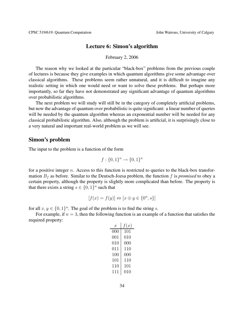
Show extracted searchable text (mathematical glyphs may differ)
CPSC 519/619: Quantum Computation John Watrous, University of Calgary
Lecture 6: Simon’s algorithm
February 2, 2006
The reason why we looked at the particular “black-box” problems from the previous couple
of lectures is because they give examples in which quantum algorithms give some advantage over
classical algorithms. These problems seem rather unnatural, and it is difficult to imagine any
realistic setting in which one would need or want to solve these problems. But perhaps more
importantly, so far they have not demonstrated any significant advantage of quantum algorithms
over probabilistic algorithms.
The next problem we will study will still be in the category of completely artificial problems,
but now the advantage of quantum over probabilistic is quite significant: a linear number of queries
will be needed by the quantum algorithm whereas an exponential number will be needed for any
classical probabilistic algorithm. Also, although the problem is artificial, it is surprisingly close to
a very natural and important real-world problem as we will see.
Simon’s problem
The input to the problem is a function of the form
f : {0, 1}n →{0, 1}n
for a positive integer n. Access to this function is restricted to queries to the black-box transfor-
mation Bf as before. Similar to the Deutsch-Jozsa problem, the function f is promised to obey a
certain property, although the property is slightly more complicated than before. The property is
that there exists a string s such that ∈{0, 1}n
[f(x) = f(y)] ⇔[x ⊕y ∈{0n, s}]
for all x, y The goal of the problem is to find the string s. ∈{0, 1}n. For example, if n = 3, then the following function is an example of a function that satisfies the
required property:
x f(x)
000 101
001 010
010 000
011 110
100 000
101 110
110 101
111 010
34
Source page 35
Direct link
Show extracted searchable text (mathematical glyphs may differ)
Specifically, the string s is 110. Every output of f occurs twice, and the two input strings corre-
sponding to any one given output have bitwise XOR equal to s = 110.
Note that the possibility that s = 0n is not ruled out—in this case the function f is simply
required to be a one-to-one function.
Intuitively this is a very hard problem classically, even if one uses randomness and accepts
a small probability of error. We will not go through the proof of this fact, because (like many
lower-bound proofs) it is harder than one might expect and I prefer that our focus remain on the
quantum algorithmic aspects of this problem. However, the intuition is reasonably simple: if you
want to solve the problem classically you need to find two different inputs x and y for which
f(x) = f(y). There is not necessarily any structure in the function f that would help you to find
two such inputs—without any additional constraints on f you are as likely to find two such inputs
by randomly guessing them as you would using any other method. But you would need to guess
Ω( √2n) different inputs before being likely to find a pair on which f takes the same output.
Simon’s algorithm
A quantum algorithm (called Simon’s Algorithm) for solving this task consists of iterating the
following quantum circuit and doing some classical post-processing:
H H H H
|0n⟩ M
H Bf H
|0n⟩
Note that the Bf gate has a different (but very similar) form from before because the input and
output of the function f are n-bit strings:
Bf |x⟩|y⟩= |x⟩|f(x) ⊕y⟩
where ⊕denotes the bitwise XOR. Before describing the classical post-processing, let us try to determine some properties of the
measurement outcome in the above circuit. The circuit begins in state |0n⟩|0n⟩, and Hadamard
35
Source page 36
Direct link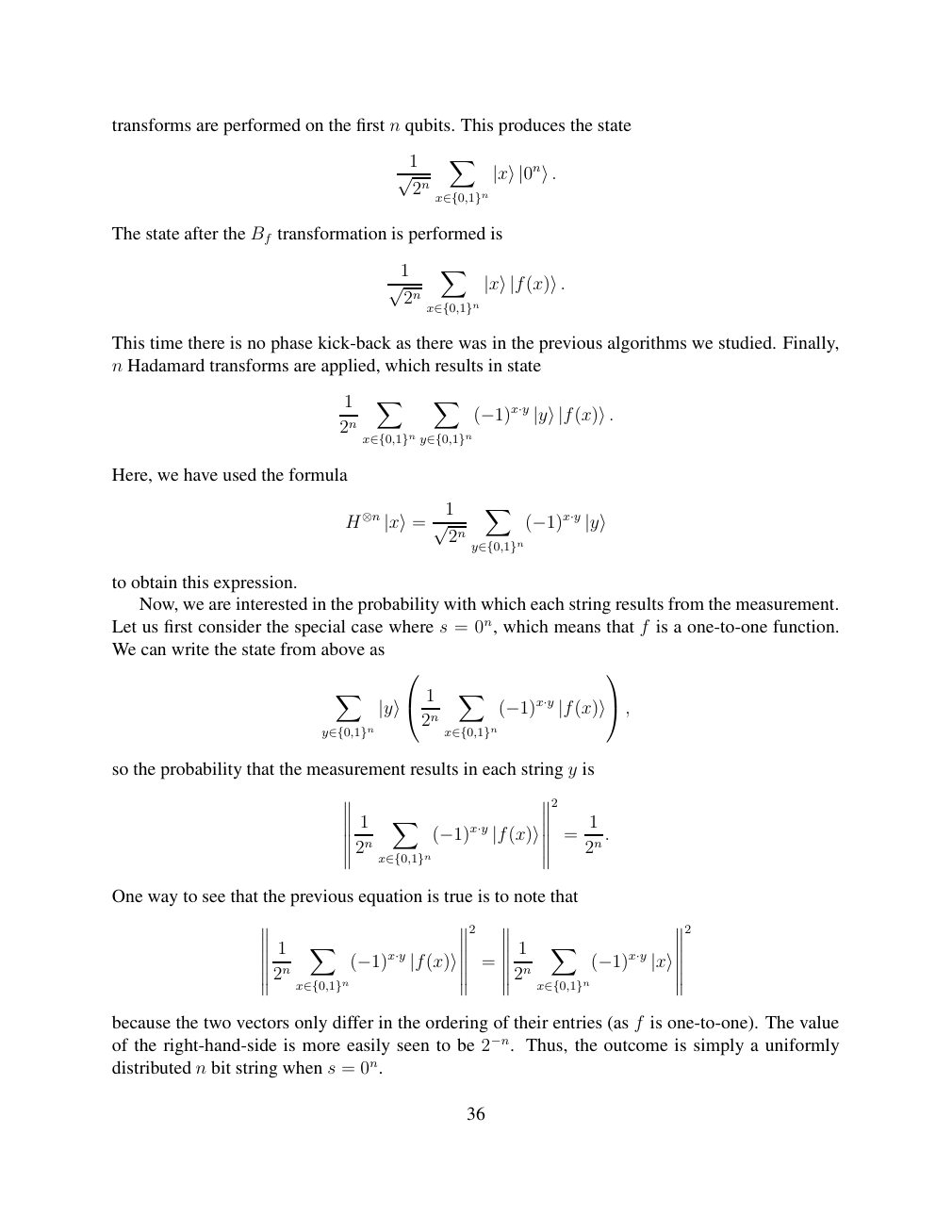
Show extracted searchable text (mathematical glyphs may differ)
transforms are performed on the first n qubits. This produces the state
X 1
√ 2n |x⟩|0n⟩.
x∈{0,1}n
The state after the Bf transformation is performed is
X 1
√ 2n |x⟩|f(x)⟩.
x∈{0,1}n
This time there is no phase kick-back as there was in the previous algorithms we studied. Finally,
n Hadamard transforms are applied, which results in state
X X 1
2n (−1)x·y |y⟩|f(x)⟩.
x∈{0,1}n y∈{0,1}n
Here, we have used the formula
X 1
H⊗n |x⟩= √ 2n (−1)x·y |y⟩
y∈{0,1}n
to obtain this expression.
Now, we are interested in the probability with which each string results from the measurement.
Let us first consider the special case where s = 0n, which means that f is a one-to-one function.
We can write the state from above as
X X
1 , |y⟩ 2n (−1)x·y |f(x)⟩
y∈{0,1}n x∈{0,1}n
so the probability that the measurement results in each string y is
2
X 1 1
= 2n (−1)x·y |f(x)⟩ 2n.
x∈{0,1}n
One way to see that the previous equation is true is to note that
2 2
X X 1 1
= 2n (−1)x·y |f(x)⟩ 2n (−1)x·y |x⟩
x∈{0,1}n x∈{0,1}n
because the two vectors only differ in the ordering of their entries (as f is one-to-one). The value
of the right-hand-side is more easily seen to be 2−n. Thus, the outcome is simply a uniformly
distributed n bit string when s = 0n.
36
Source page 37
Direct link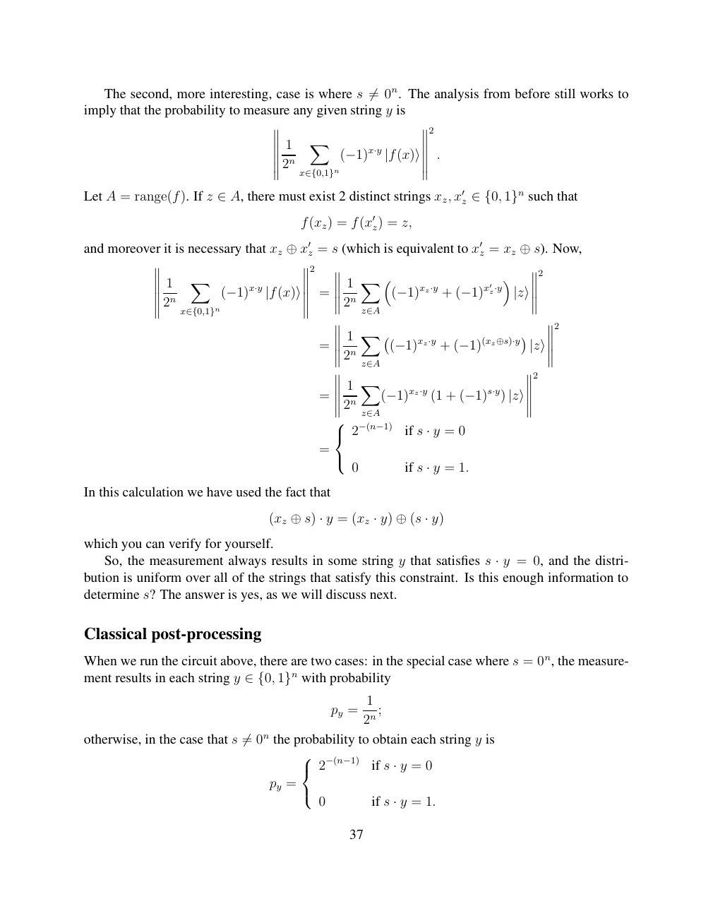
Show extracted searchable text (mathematical glyphs may differ)
The second, more interesting, case is where s 0n. The analysis from before still works to ̸=imply that the probability to measure any given string y is
2
X 1
. 2n (−1)x·y |f(x)⟩
x∈{0,1}n
Let A = range(f). If z ∈A, there must exist 2 distinct strings xz, x′z ∈{0, 1}n such that
f(xz) = f(x′z) = z,
and moreover it is necessary that xz ⊕x′ z = s (which is equivalent to x′z = xz ⊕s). Now,
2
X X 2 1 1
= + z·y 2n (−1)x·y |f(x)⟩ 2n (−1)xz·y (−1)x′ |z⟩
x∈{0,1}n z∈A
X 2 1
= + 2n (−1)xz·y (−1)(xz⊕s)·y |z⟩
z∈A
X 2 1
= (1 + 2n (−1)xz·y (−1)s·y) |z⟩
z∈A
2−(n−1) if s y = 0 ·
=
0 if s y = 1. ·
In this calculation we have used the fact that
(xz ⊕s) · y = (xz · y) ⊕(s · y)
which you can verify for yourself.
So, the measurement always results in some string y that satisfies s y = 0, and the distri- ·bution is uniform over all of the strings that satisfy this constraint. Is this enough information to
determine s? The answer is yes, as we will discuss next.
Classical post-processing
When we run the circuit above, there are two cases: in the special case where s = 0n, the measure-
ment results in each string y with probability ∈{0, 1}n
1
py = 2n;
otherwise, in the case that s 0n the probability to obtain each string y is ̸=
2−(n−1) if s y = 0 ·
py =
0 if s y = 1. ·
37
Source page 38
Direct link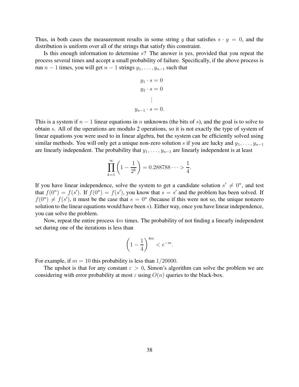
Show extracted searchable text (mathematical glyphs may differ)
Thus, in both cases the measurement results in some string y that satisfies s y = 0, and the ·distribution is uniform over all of the strings that satisfy this constraint.
Is this enough information to determine s? The answer is yes, provided that you repeat the
process several times and accept a small probability of failure. Specifically, if the above process is
run n times, you will get n strings y1, . . . , such that −1 −1 yn−1
y1 · s = 0
y2 · s = 0
...
yn−1 · s = 0.
This is a system if n linear equations in n unknowns (the bits of s), and the goal is to solve to −1obtain s. All of the operations are modulo 2 operations, so it is not exactly the type of system of
linear equations you were used to in linear algebra, but the system can be efficiently solved using
similar methods. You will only get a unique non-zero solution s if you are lucky and y1, . . . , yn−1
are linearly independent. The probability that y1, . . . , are linearly independent is at least yn−1
Y∞ 1
1 = 0.288788 > −12k · · · 4.
k=1
If you have linear independence, solve the system to get a candidate solution s′ 0n, and test ̸=that f(0n) = f(s′). If f(0n) = f(s′), you know that s = s′ and the problem has been solved. If
f(0n) f(s′), it must be the case that s = 0n (because if this were not so, the unique nonzero ̸=solution to the linear equations would have been s). Either way, once you have linear independence,
you can solve the problem.
Now, repeat the entire process 4m times. The probability of not finding a linearly independent
set during one of the iterations is less than
4m
1 < e−m. −14
For example, if m = 10 this probability is less than 1/20000.
The upshot is that for any constant ε > 0, Simon’s algorithm can solve the problem we are
considering with error probability at most ε using O(n) queries to the black-box.
38
⊗ Circuit walkthrough: entanglement and measurement
The Hadamard gate prepares (|0⟩ + |1⟩)/√2 on the first qubit. The controlled-NOT then creates the Bell state (|00⟩ + |11⟩)/√2. Measuring both qubits in the computational basis produces correlated 00 and 11 outcomes, each with ideal probability 1/2. This example illustrates a circuit building block; it is not a complete implementation of the surrounding algorithm.
Show runnable Qiskit example
from qiskit import QuantumCircuit
from qiskit_aer import AerSimulator

qc = QuantumCircuit(2, 2)
qc.h(0)             # Superpose the first qubit
qc.cx(0, 1)         # Entangle both qubits
qc.measure([0, 1], [0, 1])
print(qc.draw(output="text"))
result = AerSimulator().run(qc, shots=1024).result()
print(result.get_counts())  # Approximately 00 and 11
Install qiskit and qiskit-aer locally to execute this code. The diagram is a static circuit illustration, not a browser-based simulator.