Math fidelity: The original PDF page is displayed as a high-resolution image so that equations, bra–ket notation, matrix layouts and circuit diagrams remain exactly as in the source. The expandable text layer is for searching and may not reproduce every mathematical glyph.
Source page 14
Direct link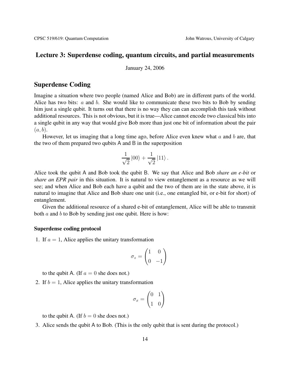
Show extracted searchable text (mathematical glyphs may differ)
CPSC 519/619: Quantum Computation John Watrous, University of Calgary
Lecture 3: Superdense coding, quantum circuits, and partial measurements
January 24, 2006
Superdense Coding
Imagine a situation where two people (named Alice and Bob) are in different parts of the world.
Alice has two bits: a and b. She would like to communicate these two bits to Bob by sending
him just a single qubit. It turns out that there is no way they can can accomplish this task without
additional resources. This is not obvious, but it is true—Alice cannot encode two classical bits into
a single qubit in any way that would give Bob more than just one bit of information about the pair
(a, b).
However, let us imaging that a long time ago, before Alice even knew what a and b are, that
the two of them prepared two qubits A and B in the superposition
1 1
√ 2 |00⟩+ √ 2 |11⟩.
Alice took the qubit A and Bob took the qubit B. We say that Alice and Bob share an e-bit or
share an EPR pair in this situation. It is natural to view entanglement as a resource as we will
see; and when Alice and Bob each have a qubit and the two of them are in the state above, it is
natural to imagine that Alice and Bob share one unit (i.e., one entangled bit, or e-bit for short) of
entanglement.
Given the additional resource of a shared e-bit of entanglement, Alice will be able to transmit
both a and b to Bob by sending just one qubit. Here is how:
Superdense coding protocol
1. If a = 1, Alice applies the unitary transformation
!
1 0
σz =
0 −1
to the qubit A. (If a = 0 she does not.)
2. If b = 1, Alice applies the unitary transformation
!
0 1
σx =
1 0
to the qubit A. (If b = 0 she does not.)
3. Alice sends the qubit A to Bob. (This is the only qubit that is sent during the protocol.)
14
Source page 15
Direct link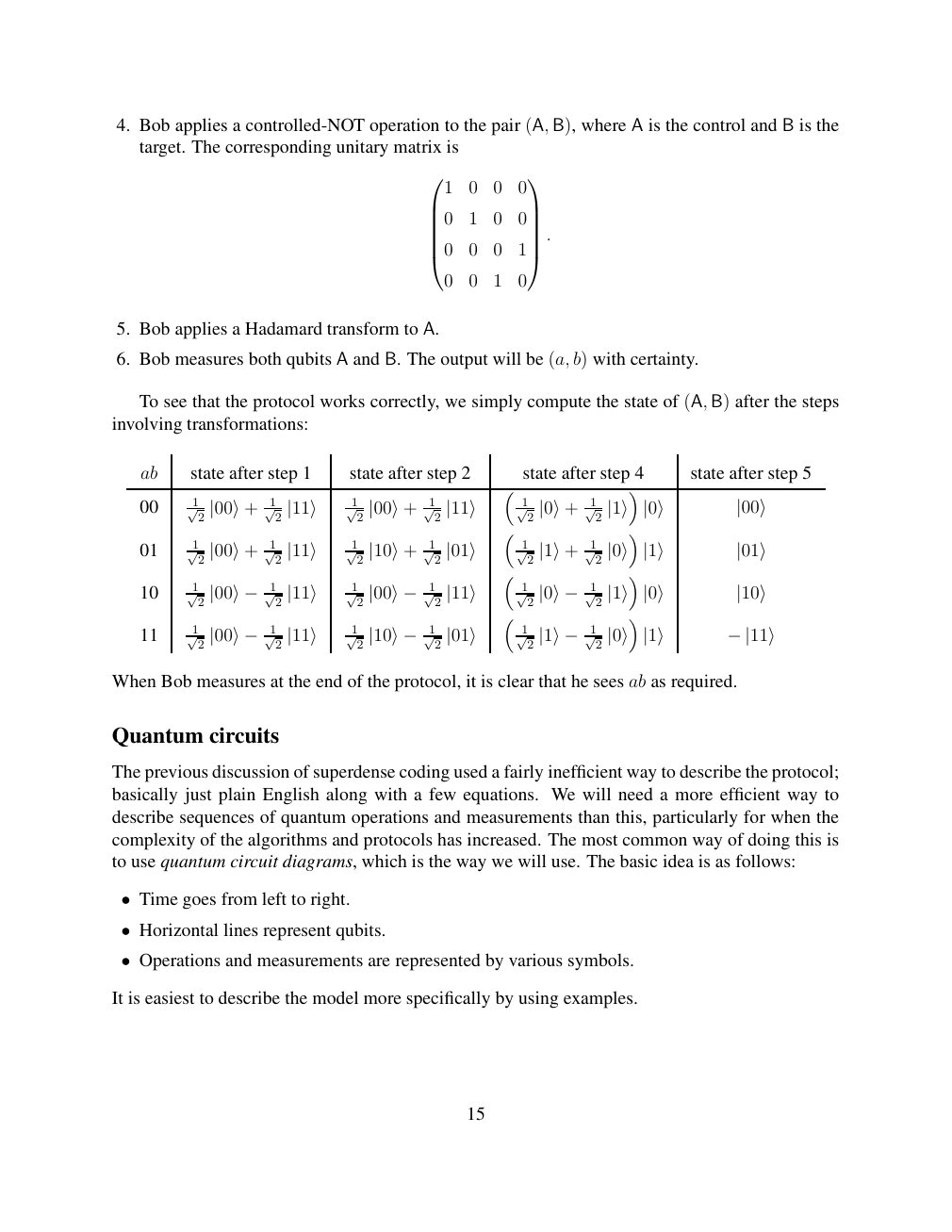
Show extracted searchable text (mathematical glyphs may differ)
4. Bob applies a controlled-NOT operation to the pair (A, B), where A is the control and B is the
target. The corresponding unitary matrix is
1 0 0 0
0 1 0 0
.
0 0 0 1
0 0 1 0
5. Bob applies a Hadamard transform to A.
6. Bob measures both qubits A and B. The output will be (a, b) with certainty.
To see that the protocol works correctly, we simply compute the state of (A, B) after the steps
involving transformations:
ab state after step 1 state after step 2 state after step 4 state after step 5
00 √12 √12 √12 √12 √12 √12 |00⟩+ |11⟩ |00⟩+ |11⟩ |0⟩+ |1⟩ |0⟩ |00⟩
01 √12 √12 √12 √12 √12 √12 |00⟩+ |11⟩ |10⟩+ |01⟩ |1⟩+ |0⟩ |1⟩ |01⟩
10 √12 √12 √12 √12 √12 √12 |00⟩− |11⟩ |00⟩− |11⟩ |0⟩− |1⟩ |0⟩ |10⟩
11 √12 √12 √12 √12 √12 √12 |00⟩− |11⟩ |10⟩− |01⟩ |1⟩− |0⟩ |1⟩ −|11⟩
When Bob measures at the end of the protocol, it is clear that he sees ab as required.
Quantum circuits
The previous discussion of superdense coding used a fairly inefficient way to describe the protocol;
basically just plain English along with a few equations. We will need a more efficient way to
describe sequences of quantum operations and measurements than this, particularly for when the
complexity of the algorithms and protocols has increased. The most common way of doing this is
to use quantum circuit diagrams, which is the way we will use. The basic idea is as follows:
Time goes from left to right. •
Horizontal lines represent qubits. •
Operations and measurements are represented by various symbols. •
It is easiest to describe the model more specifically by using examples.
15
Source page 16
Direct link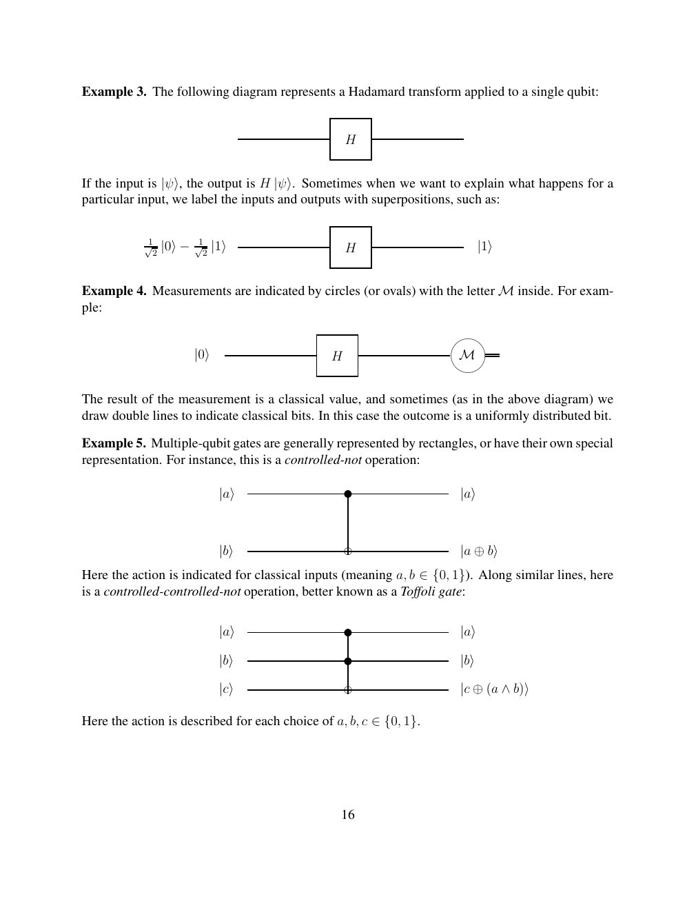
Show extracted searchable text (mathematical glyphs may differ)
Example 3. The following diagram represents a Hadamard transform applied to a single qubit:
H
HIf the input is |ψ⟩, the output is |ψ⟩. Sometimes when we want to explain what happens for aparticular input, we label the inputs and outputs with superpositions, such as:
1 1
2 |1⟩ H |1⟩ √2 |0⟩− √
Example 4. Measurements are indicated by circles (or ovals) with the letter inside. For exam- Mple:
|0⟩ H M
The result of the measurement is a classical value, and sometimes (as in the above diagram) we
draw double lines to indicate classical bits. In this case the outcome is a uniformly distributed bit.
Example 5. Multiple-qubit gates are generally represented by rectangles, or have their own special
representation. For instance, this is a controlled-not operation:
|a⟩ |a⟩
|b⟩ |a ⊕b⟩
Here the action is indicated for classical inputs (meaning a, b Along similar lines, here ∈{0, 1}).is a controlled-controlled-not operation, better known as a Toffoli gate:
|a⟩ |a⟩
|b⟩ |b⟩
|c⟩ |c ⊕(a ∧b)⟩
Here the action is described for each choice of a, b, c ∈{0, 1}.
16
Source page 17
Direct link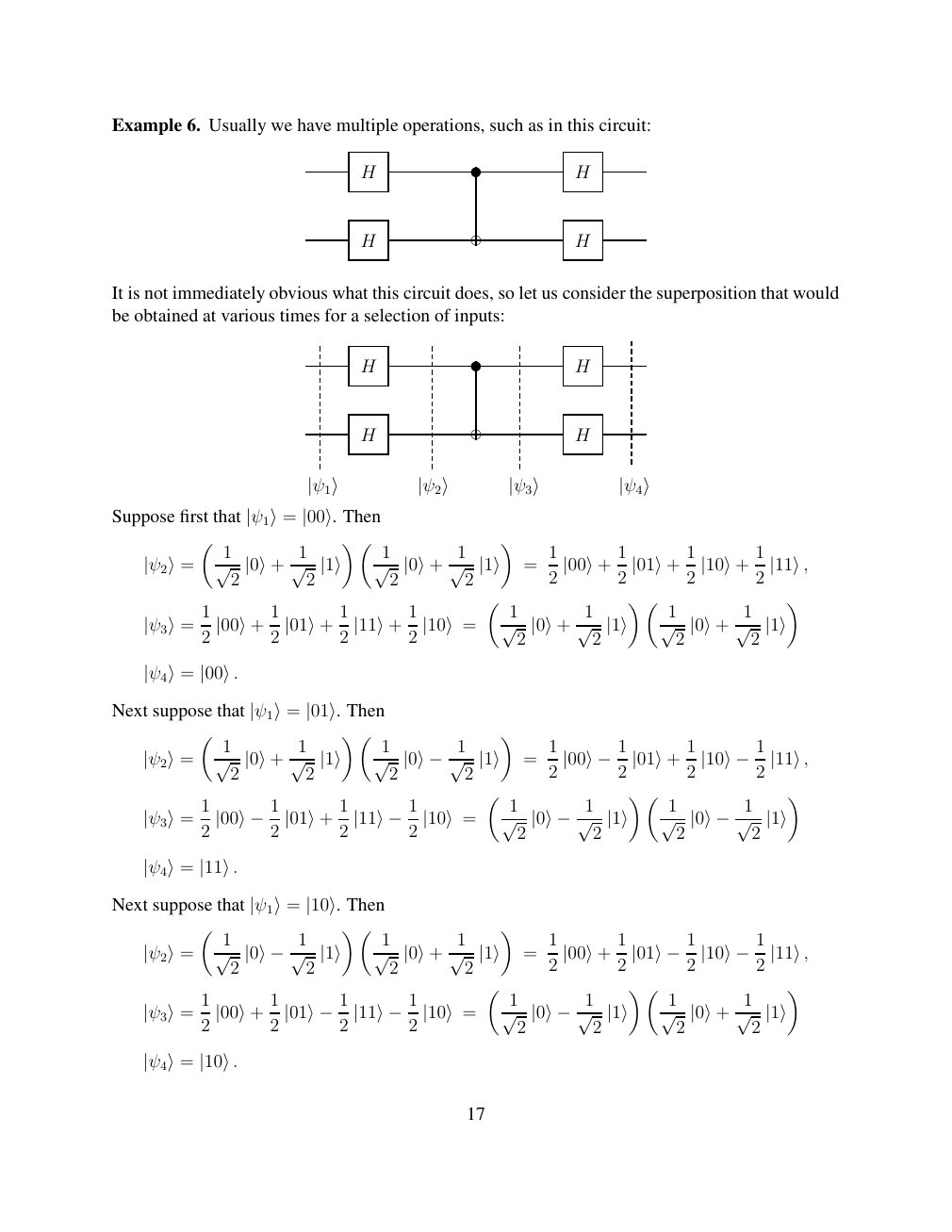
Show extracted searchable text (mathematical glyphs may differ)
Example 6. Usually we have multiple operations, such as in this circuit:
H H
H H
It is not immediately obvious what this circuit does, so let us consider the superposition that would
be obtained at various times for a selection of inputs:
H H
H H
|ψ1⟩ |ψ2⟩ |ψ3⟩ |ψ4⟩
Suppose first that Then |ψ1⟩= |00⟩.
1 1 1 1 1 1 1 1
|ψ2⟩= √ 2 |0⟩+ √ 2 |1⟩ √ 2 |0⟩+ √ 2 |1⟩ = 2 |00⟩+ 2 |01⟩+ 2 |10⟩+ 2 |11⟩,
1 1 1 1 1 1 1 1
|ψ3⟩= 2 |00⟩+ 2 |01⟩+ 2 |11⟩+ 2 |10⟩= √ 2 |0⟩+ √ 2 |1⟩ √ 2 |0⟩+ √ 2 |1⟩
|ψ4⟩= |00⟩.
Next suppose that Then |ψ1⟩= |01⟩.
1 1 1 1 1
= 2 |00⟩−12 |01⟩+ 2 |10⟩−12 |11⟩, |ψ2⟩= √ 2 |0⟩+ √ 2 |1⟩ √ 2 |0⟩−1√ 2 |1⟩
1 1 1 1
|ψ3⟩= 2 |00⟩−12 |01⟩+ 2 |11⟩−12 |10⟩= √ 2 |0⟩−1√ 2 |1⟩ √ 2 |0⟩−1√ 2 |1⟩
|ψ4⟩= |11⟩.
Next suppose that Then |ψ1⟩= |10⟩.
1 1 1 1 1
= 2 |00⟩+ 2 |01⟩−12 |10⟩−12 |11⟩, |ψ2⟩= √ 2 |0⟩−1√ 2 |1⟩ √ 2 |0⟩+ √ 2 |1⟩
1 1 1 1 1
|ψ3⟩= 2 |00⟩+ 2 |01⟩−12 |11⟩−12 |10⟩= √ 2 |0⟩−1√ 2 |1⟩ √ 2 |0⟩+ √ 2 |1⟩
|ψ4⟩= |10⟩.
17
Source page 18
Direct link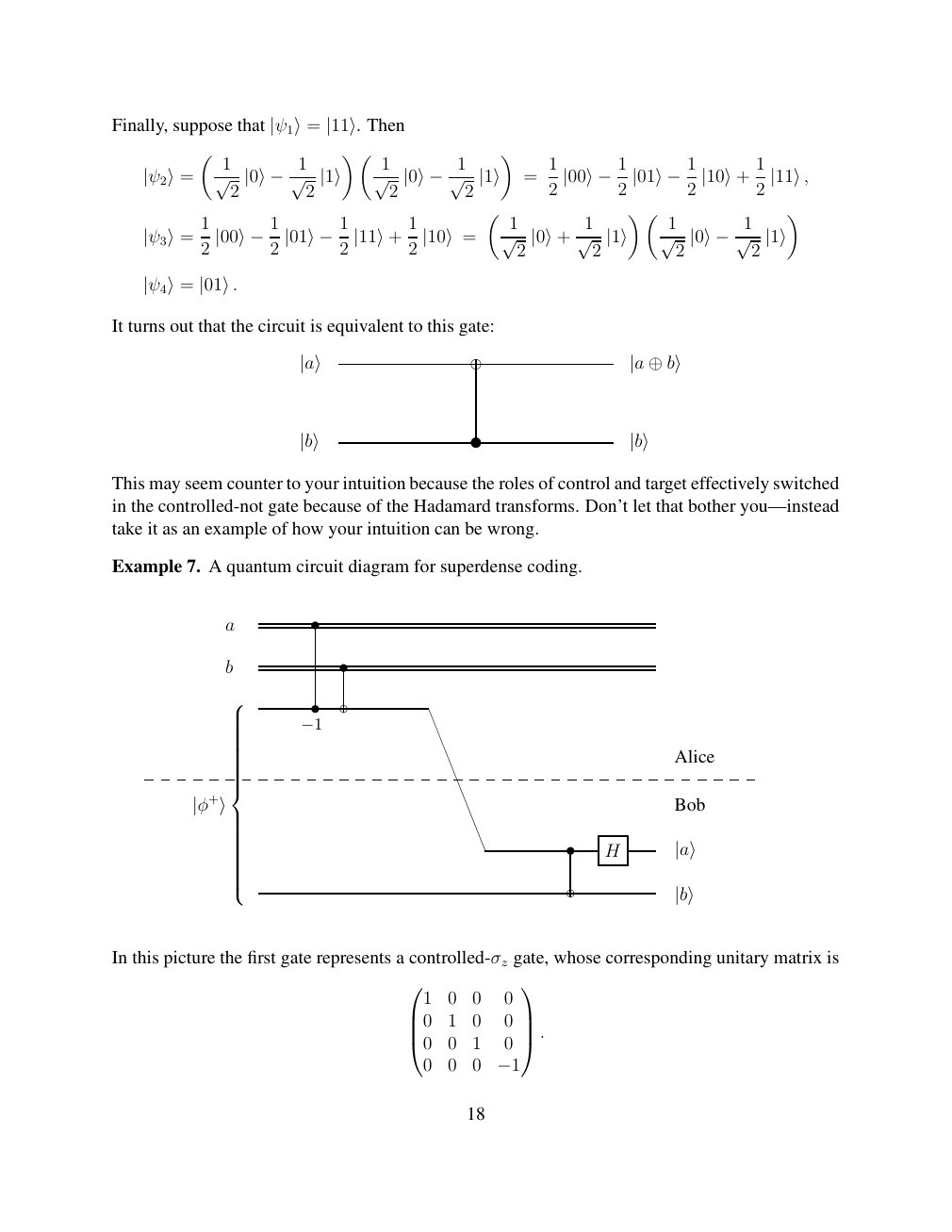
Show extracted searchable text (mathematical glyphs may differ)
Finally, suppose that Then |ψ1⟩= |11⟩.
1 1 1 1
= 2 |00⟩−12 |01⟩−12 |10⟩+ 2 |11⟩, |ψ2⟩= √ 2 |0⟩−1√ 2 |1⟩ √ 2 |0⟩−1√ 2 |1⟩
1 1 1 1 1
|ψ3⟩= 2 |00⟩−12 |01⟩−12 |11⟩+ 2 |10⟩= √ 2 |0⟩+ √ 2 |1⟩ √ 2 |0⟩−1√ 2 |1⟩
|ψ4⟩= |01⟩.
It turns out that the circuit is equivalent to this gate:
|a⟩ |a ⊕b⟩
|b⟩ |b⟩
This may seem counter to your intuition because the roles of control and target effectively switched
in the controlled-not gate because of the Hadamard transforms. Don’t let that bother you—instead
take it as an example of how your intuition can be wrong.
Example 7. A quantum circuit diagram for superdense coding.
a
b
−1 Alice
|φ+⟩ Bob H |a⟩
|b⟩
In this picture the first gate represents a controlled-σz gate, whose corresponding unitary matrix is
1 0 0 0
0 1 0 0 . 0 0 1 0
0 0 0 −1
18
Source page 19
Direct link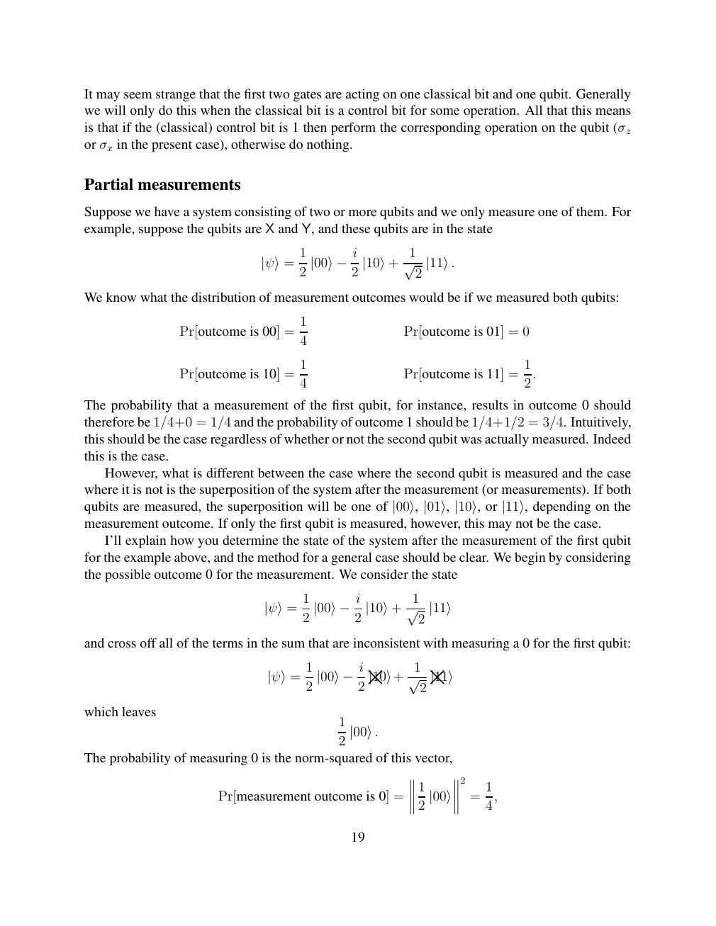
Show extracted searchable text (mathematical glyphs may differ)
It may seem strange that the first two gates are acting on one classical bit and one qubit. Generally
we will only do this when the classical bit is a control bit for some operation. All that this means
is that if the (classical) control bit is 1 then perform the corresponding operation on the qubit (σz
or σx in the present case), otherwise do nothing.
Partial measurements
Suppose we have a system consisting of two or more qubits and we only measure one of them. For
example, suppose the qubits are X and Y, and these qubits are in the state
1 1
|ψ⟩= 2 |00⟩−i2 |10⟩+ √ 2 |11⟩.
We know what the distribution of measurement outcomes would be if we measured both qubits:
1
Pr[outcome is 00] = Pr[outcome is 01] = 0
4
1 1
Pr[outcome is 10] = Pr[outcome is 11] = 4 2.
The probability that a measurement of the first qubit, for instance, results in outcome 0 should
therefore be 1/4+0 = 1/4 and the probability of outcome 1 should be 1/4+1/2 = 3/4. Intuitively,
this should be the case regardless of whether or not the second qubit was actually measured. Indeed
this is the case.
However, what is different between the case where the second qubit is measured and the case
where it is not is the superposition of the system after the measurement (or measurements). If both
qubits are measured, the superposition will be one of |00⟩, |01⟩, |10⟩, or |11⟩, depending on themeasurement outcome. If only the first qubit is measured, however, this may not be the case.
I’ll explain how you determine the state of the system after the measurement of the first qubit
for the example above, and the method for a general case should be clear. We begin by considering
the possible outcome 0 for the measurement. We consider the state
1 1
|ψ⟩= 2 |00⟩−i2 |10⟩+ √ 2 |11⟩
and cross off all of the terms in the sum that are inconsistent with measuring a 0 for the first qubit:
1 1
|11⟩ |10⟩ + √ 2 |ψ⟩= 2 |00⟩−i2× ×which leaves
1
2 |00⟩.
The probability of measuring 0 is the norm-squared of this vector,
2
1 1
Pr[measurement outcome is 0] = = 2 |00⟩ 4,
19
Source page 20
Direct link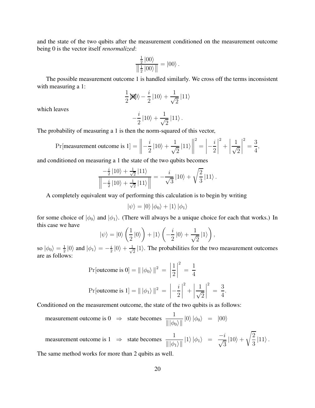
Show extracted searchable text (mathematical glyphs may differ)
and the state of the two qubits after the measurement conditioned on the measurement outcome
being 0 is the vector itself renormalized:
1
2 |00⟩ = 1 |00⟩. 2 |00⟩
The possible measurement outcome 1 is handled similarly. We cross off the terms inconsistent
with measuring a 1:
1 1
2 |00⟩ −i2 |10⟩+ √ 2 |11⟩ ×which leaves
−i2 |10⟩+ √12 |11⟩.
The probability of measuring a 1 is then the norm-squared of this vector,
2 2 2
1 1 3
Pr[measurement outcome is 1] = = + = −i2 |10⟩+ √ 2 |11⟩ −i2 √ 2 4,
and conditioned on measuring a 1 the state of the two qubits becomes
1 r
2 √2 2 −i |10⟩+ |11⟩ = 1 −i√ 3 |10⟩+ 3 |11⟩.
2 2 |10⟩+ √ −i |11⟩
A completely equivalent way of performing this calculation is to begin by writing
|ψ⟩= |0⟩|φ0⟩+ |1⟩|φ1⟩
for some choice of |φ0⟩and |φ1⟩. (There will always be a unique choice for each that works.) Inthis case we have
1 1
, |ψ⟩= |0⟩ 2 |0⟩ + |1⟩ −i2 |0⟩+ √ 2 |1⟩
so 21 2 √12 The probabilities for the two measurement outcomes |φ0⟩= |0⟩and |φ1⟩= −i |0⟩+ |1⟩.are as follows:
2
1 1
Pr[outcome is 0] = ∥|φ0⟩∥2 = 2 = 4
2 2
1 3
Pr[outcome is 1] = ∥|φ1⟩∥2 = −i2 + √ 2 = 4.
Conditioned on the measurement outcome, the state of the two qubits is as follows:
1
measurement outcome is 0 state becomes =
⇒ ∥|φ0⟩∥|0⟩|φ0⟩ |00⟩ r
1 2 measurement outcome is 1 state becomes = −i 3 |10⟩+ 3 |11⟩. ⇒ ∥|φ1⟩∥|1⟩|φ1⟩ √
The same method works for more than 2 qubits as well.
20
Source page 21
Direct link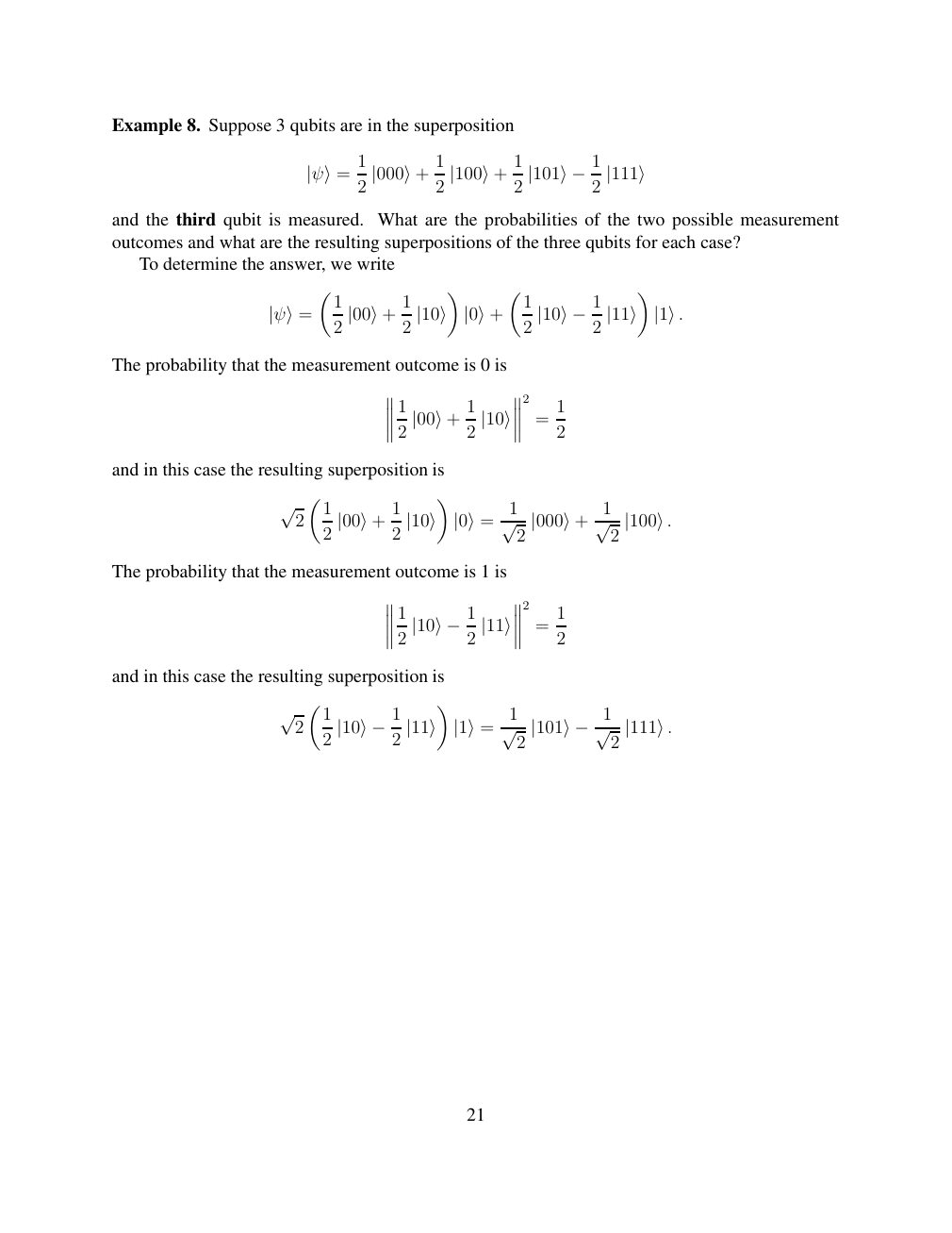
Show extracted searchable text (mathematical glyphs may differ)
Example 8. Suppose 3 qubits are in the superposition
1 1 1
|ψ⟩= 2 |000⟩+ 2 |100⟩+ 2 |101⟩−12 |111⟩
and the third qubit is measured. What are the probabilities of the two possible measurement
outcomes and what are the resulting superpositions of the three qubits for each case?
To determine the answer, we write
1 1 1
|ψ⟩= 2 |00⟩+ 2 |10⟩ |0⟩+ 2 |10⟩−12 |11⟩ |1⟩.
The probability that the measurement outcome is 0 is
2
1 1 1
= 2 |00⟩+ 2 |10⟩ 2
and in this case the resulting superposition is
√ 2 1 1 1 1 2 |00⟩+ 2 |10⟩ |0⟩= √ 2 |000⟩+ √ 2 |100⟩.
The probability that the measurement outcome is 1 is
2
1 1
= 2 |10⟩−12 |11⟩ 2
and in this case the resulting superposition is
√ 2 1 1 2 |10⟩−12 |11⟩ |1⟩= √ 2 |101⟩−1√ 2 |111⟩.
21
⊗ Circuit walkthrough: entanglement and measurement
The Hadamard gate prepares (|0⟩ + |1⟩)/√2 on the first qubit. The controlled-NOT then creates the Bell state (|00⟩ + |11⟩)/√2. Measuring both qubits in the computational basis produces correlated 00 and 11 outcomes, each with ideal probability 1/2. This example illustrates a circuit building block; it is not a complete implementation of the surrounding algorithm.
Show runnable Qiskit example
from qiskit import QuantumCircuit
from qiskit_aer import AerSimulator

qc = QuantumCircuit(2, 2)
qc.h(0)             # Superpose the first qubit
qc.cx(0, 1)         # Entangle both qubits
qc.measure([0, 1], [0, 1])
print(qc.draw(output="text"))
result = AerSimulator().run(qc, shots=1024).result()
print(result.get_counts())  # Approximately 00 and 11
Install qiskit and qiskit-aer locally to execute this code. The diagram is a static circuit illustration, not a browser-based simulator.