Math fidelity: The original PDF page is displayed as a high-resolution image so that equations, bra–ket notation, matrix layouts and circuit diagrams remain exactly as in the source. The expandable text layer is for searching and may not reproduce every mathematical glyph.
Source page 61
Direct link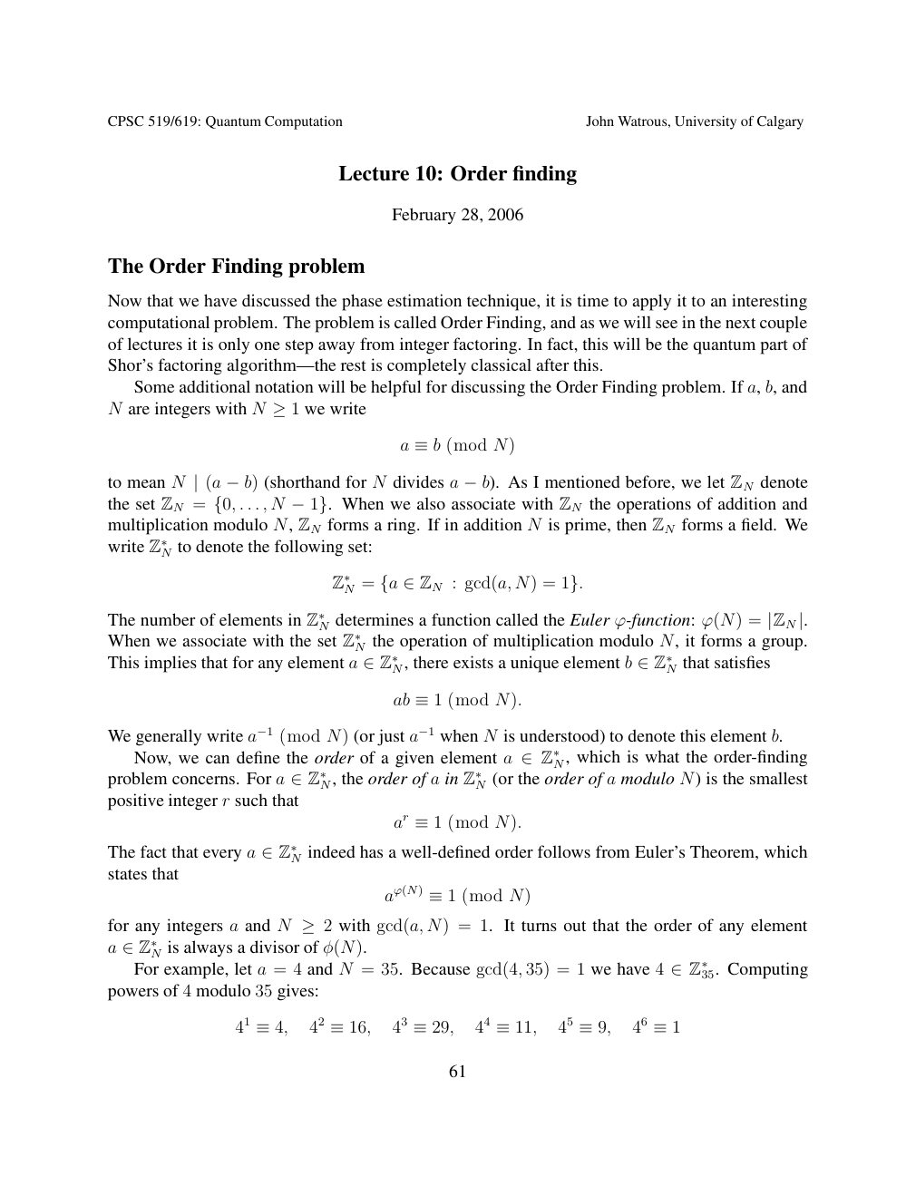
Show extracted searchable text (mathematical glyphs may differ)
CPSC 519/619: Quantum Computation John Watrous, University of Calgary
Lecture 10: Order finding
February 28, 2006
The Order Finding problem
Now that we have discussed the phase estimation technique, it is time to apply it to an interesting
computational problem. The problem is called Order Finding, and as we will see in the next couple
of lectures it is only one step away from integer factoring. In fact, this will be the quantum part of
Shor’s factoring algorithm—the rest is completely classical after this.
Some additional notation will be helpful for discussing the Order Finding problem. If a, b, and
N are integers with N we write ≥1
a ≡b (mod N)
to mean N (a (shorthand for N divides a As I mentioned before, we let ZN denote | −b) −b).the set ZN = . . . , N When we also associate with ZN the operations of addition and {0, −1}.multiplication modulo N, ZN forms a ring. If in addition N is prime, then ZN forms a field. We
write Z∗N to denote the following set:
Z∗N = {a ∈ZN : gcd(a, N) = 1}.
The number of elements in Z∗N determines a function called the Euler ϕ-function: ϕ(N) = |ZN |.When we associate with the set Z∗N the operation of multiplication modulo N, it forms a group.
N that satisfiesThis implies that for any element a ∈Z∗N, there exists a unique element b ∈Z∗
ab ≡1 (mod N).
We generally write a−1 (mod N) (or just a−1 when N is understood) to denote this element b.
Now, we can define the order of a given element a ∈Z∗N, which is what the order-finding a in Z∗N (or the order of a modulo N) is the smallestproblem concerns. For a ∈Z∗N, the order ofpositive integer r such that
ar ≡1 (mod N).
N indeed has a well-defined order follows from Euler’s Theorem, whichThe fact that every a ∈Z∗states that
aϕ(N) ≡1 (mod N)
for any integers a and N with gcd(a, N) = 1. It turns out that the order of any element ≥2 N is always a divisor of φ(N).a ∈Z∗
For example, let a = 4 and N = 35. Because gcd(4, 35) = 1 we have 4 ∈Z∗35. Computingpowers of 4 modulo 35 gives:
41 ≡4, 42 ≡16, 43 ≡29, 44 ≡11, 45 ≡9, 46 ≡1
61
Source page 62
Direct link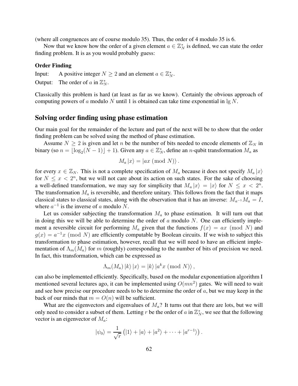
Show extracted searchable text (mathematical glyphs may differ)
(where all congruences are of course modulo 35). Thus, the order of 4 modulo 35 is 6.
N is defined, we can state the order Now that we know how the order of a given element a ∈Z∗finding problem. It is as you would probably guess:
Order Finding
Input: A positive integer N and an element a N. ≥2 ∈Z∗
Output: The order of a in Z∗N.
Classically this problem is hard (at least as far as we know). Certainly the obvious approach of
computing powers of a modulo N until 1 is obtained can take time exponential in lg N.
Solving order finding using phase estimation
Our main goal for the remainder of the lecture and part of the next will be to show that the order
finding problem can be solved using the method of phase estimation.
Assume N is given and let n be the number of bits needed to encode elements of ZN in ≥2binary (so n = 1). Given any a N, define an n-qubit transformation Ma as ⌊log2(N −1)⌋+ ∈Z∗
Ma |x⟩= |ax (mod N)⟩.
Ma because it does not specify Mafor every x ∈ZN. This is not a complete specification of |x⟩for N < 2n, but we will not care about its action on such states. For the sake of choosing ≤xa well-defined transformation, we may say for simplicity that Ma N < 2n. |x⟩= |x⟩for ≤xThe transformation Ma is reversible, and therefore unitary. This follows from the fact that it maps
classical states to classical states, along with the observation that it has an inverse: Ma−1Ma = I,
where a−1 is the inverse of a modulo N.
Let us consider subjecting the transformation Ma to phase estimation. It will turn out that
in doing this we will be able to determine the order of a modulo N. One can efficiently imple-
ment a reversible circuit for performing Ma given that the functions f(x) = ax (mod N) and
g(x) = a−1x (mod N) are efficiently computable by Boolean circuits. If we wish to subject this
transformation to phase estimation, however, recall that we will need to have an efficient imple-
mentation of Λm(Ma) for m (roughly) corresponding to the number of bits of precision we need.
In fact, this transformation, which can be expressed as
Λm(Ma) |k⟩|x⟩= |k⟩|akx (mod N)⟩,
can also be implemented efficiently. Specifically, based on the modular exponentiation algorithm I
mentioned several lectures ago, it can be implemented using O(mn2) gates. We will need to wait
and see how precise our procedure needs to be to determine the order of a, but we may keep in the
back of our minds that m = O(n) will be sufficient.
What are the eigenvectors and eigenvalues of Ma? It turns out that there are lots, but we will
only need to consider a subset of them. Letting r be the order of a in Z∗N, we see that the following
vector is an eigenvector of Ma:
1
|ψ0⟩= √r |1⟩+ |a⟩+ |a2⟩+ · · · + |ar−1⟩ .
62
Source page 63
Direct link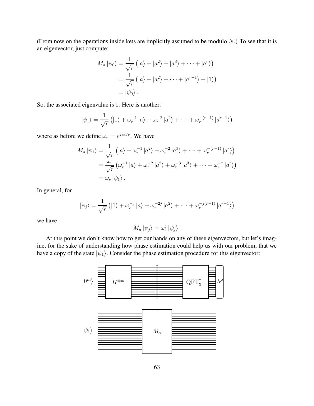
Show extracted searchable text (mathematical glyphs may differ)
(From now on the operations inside kets are implicitly assumed to be modulo N.) To see that it is
an eigenvector, just compute:
1
Ma |ψ0⟩= √r |a⟩+ |a2⟩+ |a3⟩+ · · · + |ar⟩
1
= √r |a⟩+ |a2⟩+ · · · + |ar−1⟩+ |1⟩
= |ψ0⟩.
So, the associated eigenvalue is 1. Here is another:
1
r r r |ar−1⟩ |a2⟩+ · · · + ω−(r−1) |a⟩+ ω−2 |ψ1⟩= √r |1⟩+ ω−1
where as before we define ωr = e2πi/r. We have
1
r r r Ma |ψ1⟩= √r |a⟩+ ω−1 |a2⟩+ ω−2 |a3⟩+ · · · + ω−(r−1) |ar⟩
ωr
r r r r = √r ω−1 |a⟩+ ω−2 |a2⟩+ ω−3 |a3⟩+ · · · + ω−r |ar⟩
= ωr |ψ1⟩.
In general, for
1
r r r |ψj⟩= √r |1⟩+ ω−j |a⟩+ ω−2j |a2⟩+ · · · + ω−j(r−1) |ar−1⟩
we have
r Ma |ψj⟩= ωj |ψj⟩.
At this point we don’t know how to get our hands on any of these eigenvectors, but let’s imag-
ine, for the sake of understanding how phase estimation could help us with our problem, that we
have a copy of the state |ψ1⟩. Consider the phase estimation procedure for this eigenvector:
2m M |0m⟩ H⊗m QFT†
|ψ1⟩ Ma
63
Source page 64
Direct link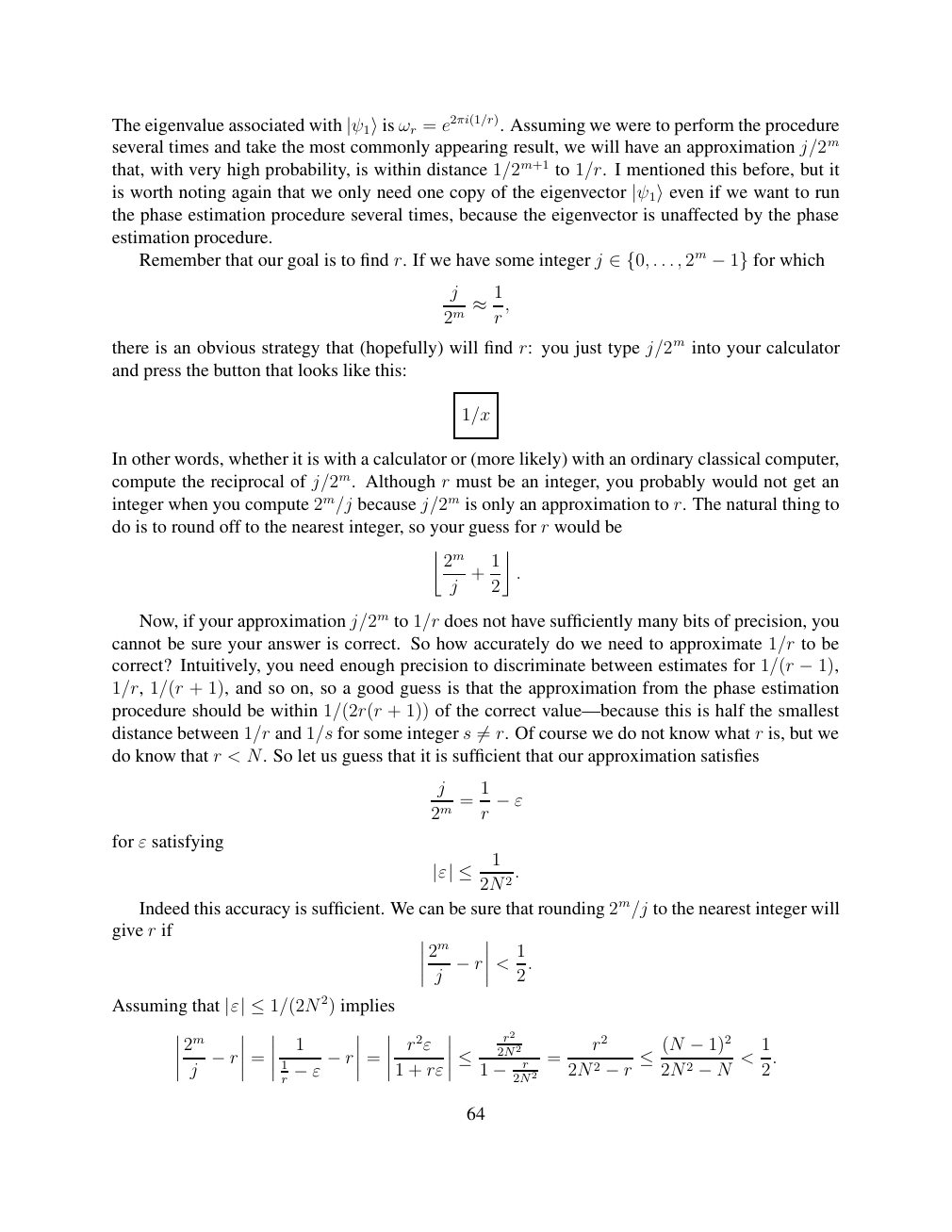
Show extracted searchable text (mathematical glyphs may differ)
ωr = e2πi(1/r). Assuming we were to perform the procedureThe eigenvalue associated with |ψ1⟩isseveral times and take the most commonly appearing result, we will have an approximation j/2m
that, with very high probability, is within distance 1/2m+1 to 1/r. I mentioned this before, but it
is worth noting again that we only need one copy of the eigenvector |ψ1⟩even if we want to runthe phase estimation procedure several times, because the eigenvector is unaffected by the phase
estimation procedure.
Remember that our goal is to find r. If we have some integer j . . . , 2m for which ∈{0, −1}
j
2m ≈1r,
there is an obvious strategy that (hopefully) will find r: you just type j/2m into your calculator
and press the button that looks like this:
1/x
In other words, whether it is with a calculator or (more likely) with an ordinary classical computer,
compute the reciprocal of j/2m. Although r must be an integer, you probably would not get an
integer when you compute 2m/j because j/2m is only an approximation to r. The natural thing to
do is to round off to the nearest integer, so your guess for r would be
2m 1
+ .
j 2
Now, if your approximation j/2m to 1/r does not have sufficiently many bits of precision, you
cannot be sure your answer is correct. So how accurately do we need to approximate 1/r to be
correct? Intuitively, you need enough precision to discriminate between estimates for 1/(r −1),1/r, 1/(r + 1), and so on, so a good guess is that the approximation from the phase estimation
procedure should be within 1/(2r(r + 1)) of the correct value—because this is half the smallest
distance between 1/r and 1/s for some integer s r. Of course we do not know what r is, but we ̸=do know that r < N. So let us guess that it is sufficient that our approximation satisfies
j 1
= 2m r −ε
for ε satisfying
1
|ε| ≤ 2N 2.
Indeed this accuracy is sufficient. We can be sure that rounding 2m/j to the nearest integer will
give r if
2m 1
< j −r 2.
Assuming that 2) implies |ε| ≤1/(2N
2m 1 r2ε 2N2r2 r2 1 −1)2 < = 1 = r = 2 2 j −r 2N ≤(N2N 2. −r 1 + rε ≤ 1 2N2 r −ε − −r −N
64
Source page 65
Direct link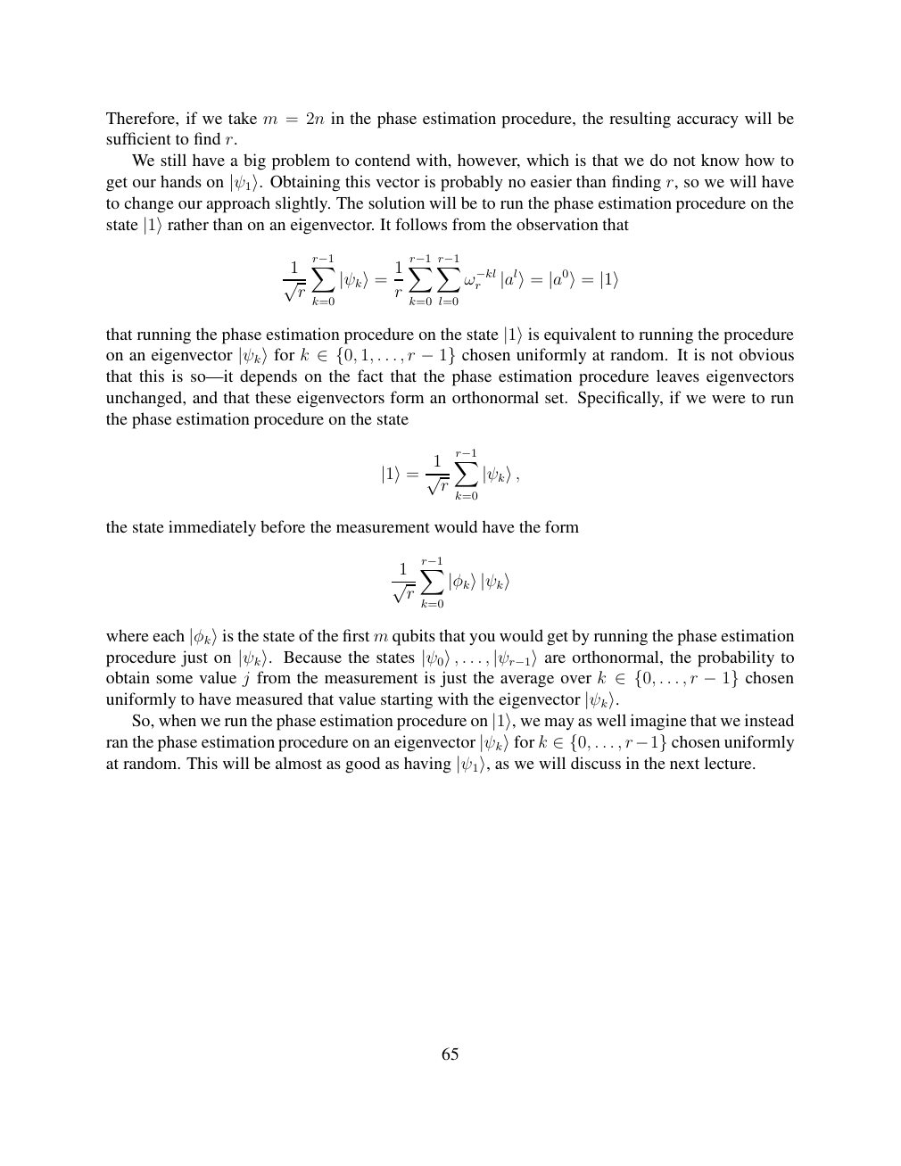
Show extracted searchable text (mathematical glyphs may differ)
Therefore, if we take m = 2n in the phase estimation procedure, the resulting accuracy will be
sufficient to find r.
We still have a big problem to contend with, however, which is that we do not know how to
get our hands on |ψ1⟩. Obtaining this vector is probably no easier than finding r, so we will haveto change our approach slightly. The solution will be to run the phase estimation procedure on the
state |1⟩rather than on an eigenvector. It follows from the observation that
Xr−1 1 Xr−1 Xr−1 1
r |al⟩= |a0⟩= |1⟩ √r |ψk⟩= r ω−kl
k=0 k=0 l=0
that running the phase estimation procedure on the state |1⟩is equivalent to running the procedure chosen uniformly at random. It is not obviouson an eigenvector |ψk⟩for k ∈{0, 1, . . ., r −1}that this is so—it depends on the fact that the phase estimation procedure leaves eigenvectors
unchanged, and that these eigenvectors form an orthonormal set. Specifically, if we were to run
the phase estimation procedure on the state
Xr−1 1
|1⟩= √r |ψk⟩,
k=0
the state immediately before the measurement would have the form
Xr−1 1
√r |φk⟩|ψk⟩
k=0
m qubits that you would get by running the phase estimationwhere each |φk⟩is the state of the first
. . . ,procedure just on |ψk⟩. Because the states |ψ0⟩, |ψr−1⟩are orthonormal, the probability toobtain some value j from the measurement is just the average over k . . . , r chosen ∈{0, −1}
uniformly to have measured that value starting with the eigenvector |ψk⟩.
So, when we run the phase estimation procedure on |1⟩, we may as well imagine that we instead chosen uniformlyran the phase estimation procedure on an eigenvector |ψk⟩for k ∈{0, . . . , r−1}
at random. This will be almost as good as having |ψ1⟩, as we will discuss in the next lecture.
65
⊗ Circuit walkthrough: entanglement and measurement
The Hadamard gate prepares (|0⟩ + |1⟩)/√2 on the first qubit. The controlled-NOT then creates the Bell state (|00⟩ + |11⟩)/√2. Measuring both qubits in the computational basis produces correlated 00 and 11 outcomes, each with ideal probability 1/2. This example illustrates a circuit building block; it is not a complete implementation of the surrounding algorithm.
Show runnable Qiskit example
from qiskit import QuantumCircuit
from qiskit_aer import AerSimulator

qc = QuantumCircuit(2, 2)
qc.h(0)             # Superpose the first qubit
qc.cx(0, 1)         # Entangle both qubits
qc.measure([0, 1], [0, 1])
print(qc.draw(output="text"))
result = AerSimulator().run(qc, shots=1024).result()
print(result.get_counts())  # Approximately 00 and 11
Install qiskit and qiskit-aer locally to execute this code. The diagram is a static circuit illustration, not a browser-based simulator.