Math fidelity: The original PDF page is displayed as a high-resolution image so that equations, bra–ket notation, matrix layouts and circuit diagrams remain exactly as in the source. The expandable text layer is for searching and may not reproduce every mathematical glyph.
Source page 6
Direct link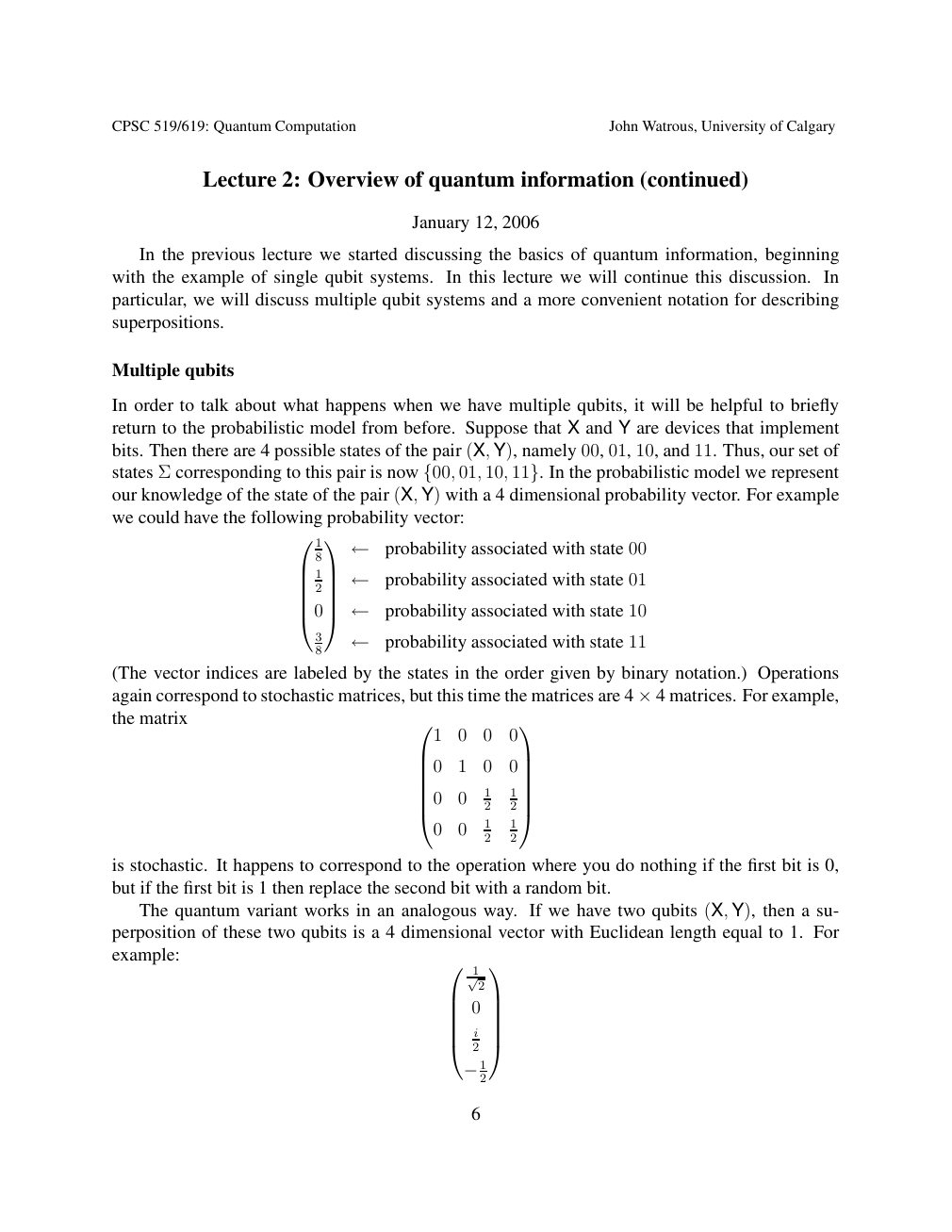
Show extracted searchable text (mathematical glyphs may differ)
CPSC 519/619: Quantum Computation John Watrous, University of Calgary
Lecture 2: Overview of quantum information (continued)
January 12, 2006
In the previous lecture we started discussing the basics of quantum information, beginning
with the example of single qubit systems. In this lecture we will continue this discussion. In
particular, we will discuss multiple qubit systems and a more convenient notation for describing
superpositions.
Multiple qubits
In order to talk about what happens when we have multiple qubits, it will be helpful to briefly
return to the probabilistic model from before. Suppose that X and Y are devices that implement
bits. Then there are 4 possible states of the pair (X, Y), namely 00, 01, 10, and 11. Thus, our set of
states Σ corresponding to this pair is now 01, 10, In the probabilistic model we represent {00, 11}.our knowledge of the state of the pair (X, Y) with a 4 dimensional probability vector. For example
we could have the following probability vector:
1 8 probability associated with state ← 00 1 probability associated with state 01 2 ← 0 probability associated with state 10 ←
3 8 probability associated with state ← 11
(The vector indices are labeled by the states in the order given by binary notation.) Operations
again correspond to stochastic matrices, but this time the matrices are 4 4 matrices. For example, ×the matrix
1 0 0 0
0 1 0 0
1 1 0 0
2 2
0 0 1 1 2 2
is stochastic. It happens to correspond to the operation where you do nothing if the first bit is 0,
but if the first bit is 1 then replace the second bit with a random bit.
The quantum variant works in an analogous way. If we have two qubits (X, Y), then a su-
perposition of these two qubits is a 4 dimensional vector with Euclidean length equal to 1. For
example: 1
√2
0
i
2
2 −1
6
Source page 7
Direct link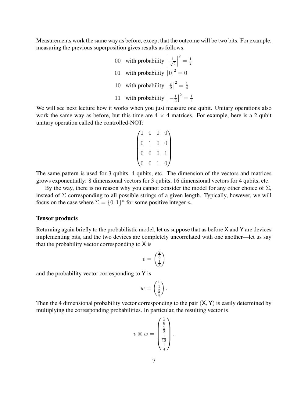
Show extracted searchable text (mathematical glyphs may differ)
Measurements work the same way as before, except that the outcome will be two bits. For example,
measuring the previous superposition gives results as follows:
2
= 1 2 00 with probability √12
= 0 01 with probability |0|2
i 2 1 = 10 with probability 2 4
2 1 = 2 4 11 with probability −1
We will see next lecture how it works when you just measure one qubit. Unitary operations also
work the same way as before, but this time are 4 4 matrices. For example, here is a 2 qubit ×unitary operation called the controlled-NOT:
1 0 0 0
0 1 0 0
0 0 0 1
0 0 1 0
The same pattern is used for 3 qubits, 4 qubits, etc. The dimension of the vectors and matrices
grows exponentially: 8 dimensional vectors for 3 qubits, 16 dimensional vectors for 4 qubits, etc.
By the way, there is no reason why you cannot consider the model for any other choice of Σ,
instead of Σ corresponding to all possible strings of a given length. Typically, however, we will
focus on the case where Σ = for some positive integer n. {0, 1}n
Tensor products
Returning again briefly to the probabilistic model, let us suppose that as before X and Y are devices
implementing bits, and the two devices are completely uncorrelated with one another—let us say
that the probability vector corresponding to X is
2
v = 31
3
and the probability vector corresponding to Y is
1
w = 43 .
4
Then the 4 dimensional probability vector corresponding to the pair (X, Y) is easily determined by
multiplying the corresponding probabilities. In particular, the resulting vector is
1
6
1
2
v ⊗w = 1 . 12
1
4
7
Source page 8
Direct link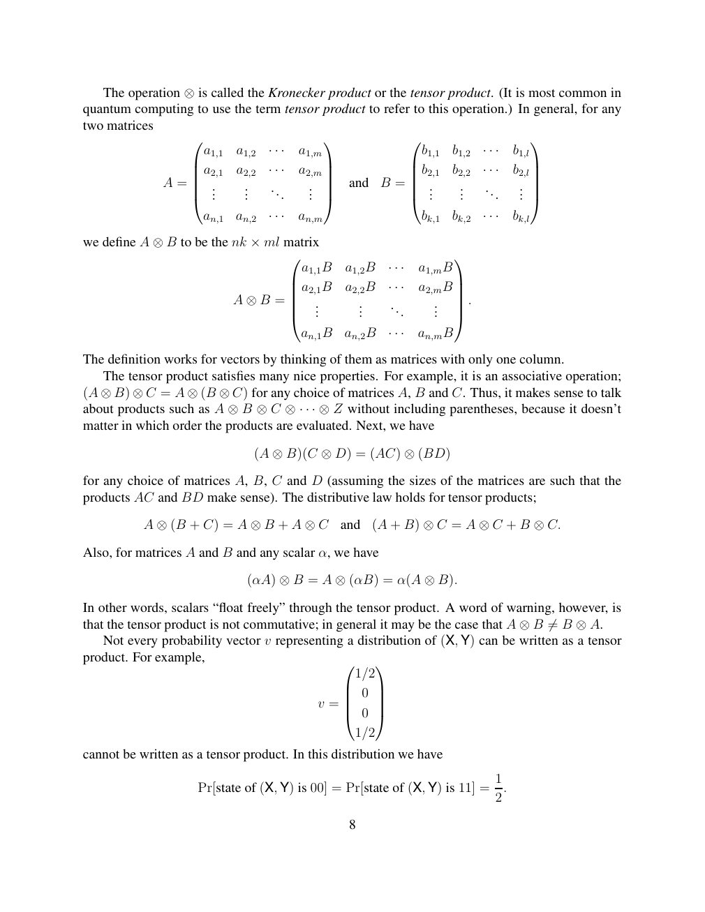
Show extracted searchable text (mathematical glyphs may differ)
The operation ⊗is called the Kronecker product or the tensor product. (It is most common inquantum computing to use the term tensor product to refer to this operation.) In general, for any
two matrices
a1,1 a1,2 · · · a1,m b1,1 b1,2 · · · b1,l
a2,1 a2,2 a2,m b2,1 b2,2 b2,l · · · · · · A = and B = ... ... ... ... ... ... ... ...
an,1 an,2 · · · an,m bk,1 bk,2 · · · bk,l
we define A to be the nk ml matrix ⊗B ×
a1,1B a1,2B · · · a1,mB
a2,1B a2,2B a2,mB · · · . A = ⊗B ... ... ... ...
an,1B an,2B · · · an,mB
The definition works for vectors by thinking of them as matrices with only one column.
The tensor product satisfies many nice properties. For example, it is an associative operation;
(A = A for any choice of matrices A, B and C. Thus, it makes sense to talk ⊗B) ⊗C ⊗(B ⊗C)about products such as A without including parentheses, because it doesn’t ⊗B ⊗C ⊗· · · ⊗Zmatter in which order the products are evaluated. Next, we have
(A ⊗B)(C ⊗D) = (AC) ⊗(BD)
for any choice of matrices A, B, C and D (assuming the sizes of the matrices are such that the
products AC and BD make sense). The distributive law holds for tensor products;
A + C) = A + A and (A + B) = A + B ⊗(B ⊗B ⊗C ⊗C ⊗C ⊗C.
Also, for matrices A and B and any scalar α, we have
(αA) ⊗B = A ⊗(αB) = α(A ⊗B).
In other words, scalars “float freely” through the tensor product. A word of warning, however, is
that the tensor product is not commutative; in general it may be the case that A B ⊗B ̸= ⊗A. Not every probability vector v representing a distribution of (X, Y) can be written as a tensor
product. For example,
1/2
0
v =
0
1/2
cannot be written as a tensor product. In this distribution we have
1
Pr[state of (X, Y) is 00] = Pr[state of (X, Y) is 11] = 2.
8
Source page 9
Direct link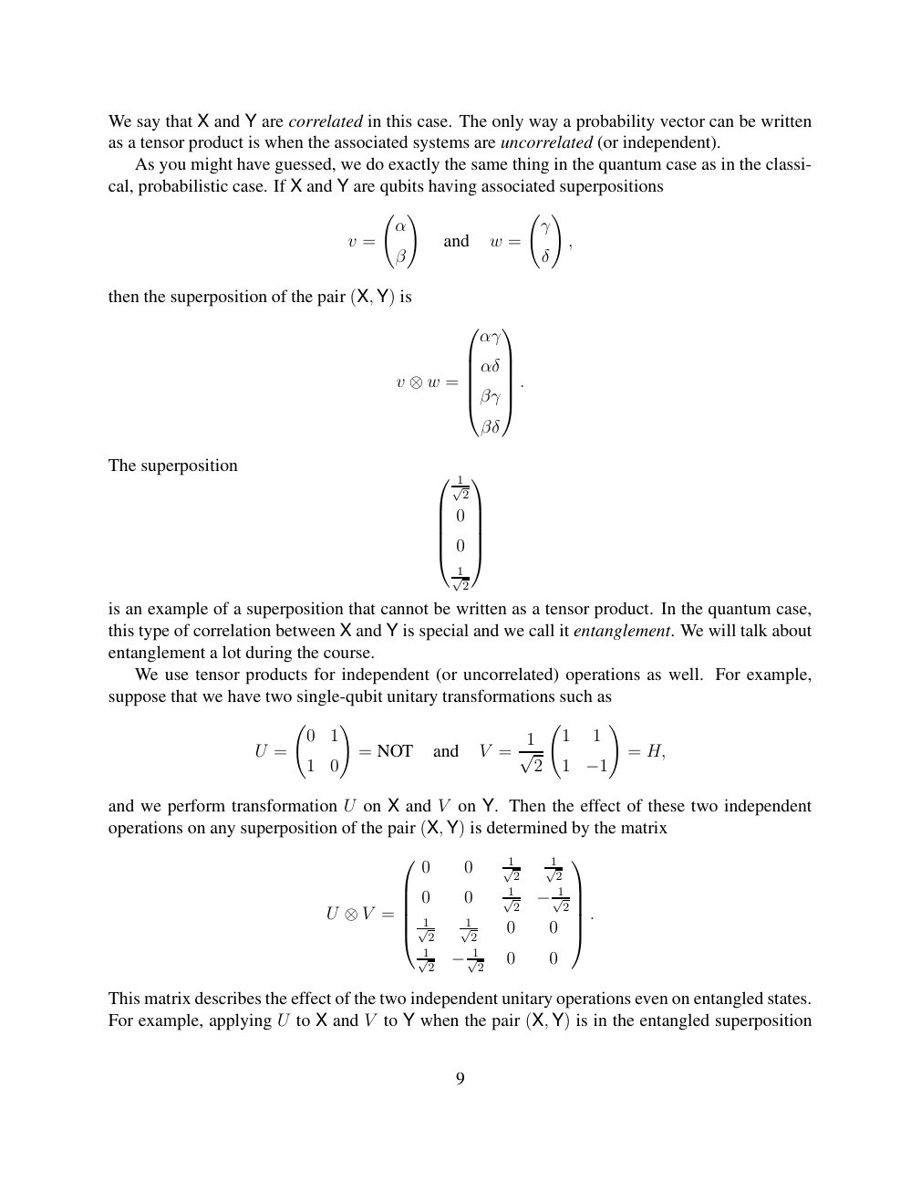
Show extracted searchable text (mathematical glyphs may differ)
We say that X and Y are correlated in this case. The only way a probability vector can be written
as a tensor product is when the associated systems are uncorrelated (or independent).
As you might have guessed, we do exactly the same thing in the quantum case as in the classi-
cal, probabilistic case. If X and Y are qubits having associated superpositions
! !
α γ
v = and w = ,
β δ
then the superposition of the pair (X, Y) is
αγ
αδ
v = . ⊗w βγ
βδ
The superposition
1
√2
0
0
1
√2
is an example of a superposition that cannot be written as a tensor product. In the quantum case,
this type of correlation between X and Y is special and we call it entanglement. We will talk about
entanglement a lot during the course.
We use tensor products for independent (or uncorrelated) operations as well. For example,
suppose that we have two single-qubit unitary transformations such as
! !
0 1 1 1 1
U = = NOT and V = = H, 1 0 √ 2 1 −1
and we perform transformation U on X and V on Y. Then the effect of these two independent
operations on any superposition of the pair (X, Y) is determined by the matrix
1 1
0 0 √2 √2
1
0 0 √2 √2 −1 . U = 1 1
0 0 ⊗V √2 √2
1 0 0 √2 √2 −1
This matrix describes the effect of the two independent unitary operations even on entangled states.
For example, applying U to X and V to Y when the pair (X, Y) is in the entangled superposition
9
Source page 10
Direct link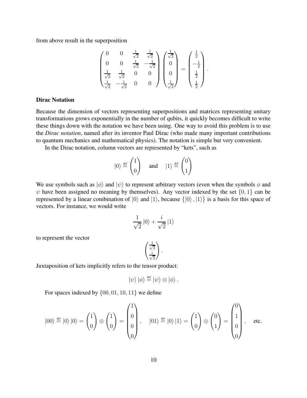
Show extracted searchable text (mathematical glyphs may differ)
from above result in the superposition
1 1 1 1
0 0 √2 √2 √2 2
1
0 0 √2 √2 0 2 −1 . −1 = 1 1 1
√2 √2 0 0 0 2
1 0 0 1 1 √2 √2 √2 2 −1
Dirac Notation
Because the dimension of vectors representing superpositions and matrices representing unitary
transformations grows exponentially in the number of qubits, it quickly becomes difficult to write
these things down with the notation we have been using. One way to avoid this problem is to use
the Dirac notation, named after its inventor Paul Dirac (who made many important contributions
to quantum mechanics and mathematical physics). The notation is simple but very convenient.
In the Dirac notation, column vectors are represented by “kets”, such as
! !
1 0
def= and def= |0⟩ 0 |1⟩ 1
φ andWe use symbols such as |φ⟩and |ψ⟩to represent arbitrary vectors (even when the symbolsψ have been assigned no meaning by themselves). Any vector indexed by the set can be {0, 1}
represented by a linear combination of |0⟩and |1⟩, because {|0⟩, |1⟩} is a basis for this space ofvectors. For instance, we would write
1 i
√ 2 |0⟩+ √ 2 |1⟩
to represent the vector !
1
√2
. i
√2
Juxtaposition of kets implicitly refers to the tensor product:
def= |ψ⟩|φ⟩ |ψ⟩⊗|φ⟩.
For spaces indexed by 01, 10, we define {00, 11}
1 0
! ! ! !
1 1 0 1 0 1
def= = , def= = , etc. |00⟩ |0⟩|0⟩= 0 ⊗ 0 0 |01⟩ |0⟩|1⟩= 0 ⊗ 1 0
0 0
10
Source page 11
Direct link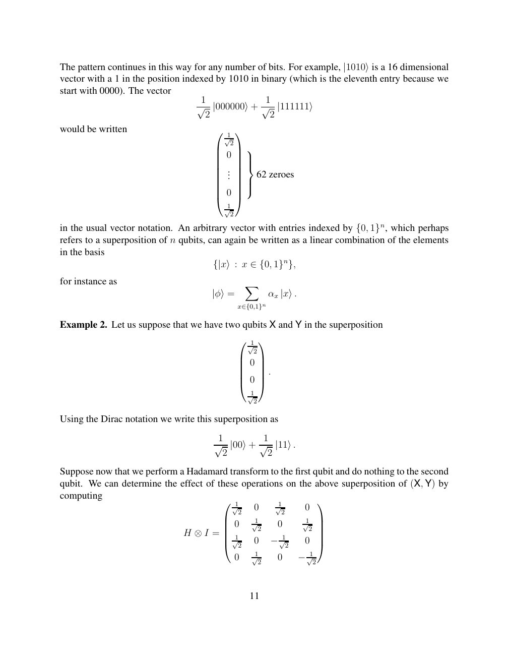
Show extracted searchable text (mathematical glyphs may differ)
The pattern continues in this way for any number of bits. For example, |1010⟩is a 16 dimensionalvector with a 1 in the position indexed by 1010 in binary (which is the eleventh entry because we
start with 0000). The vector
1 1
√ 2 |000000⟩+ √ 2 |111111⟩
would be written 1
√2
0
62 zeroes ... 0
1
√2
in the usual vector notation. An arbitrary vector with entries indexed by which perhaps {0, 1}n,refers to a superposition of n qubits, can again be written as a linear combination of the elements
in the basis
{|x⟩: x ∈{0, 1}n},
for instance as X
|φ⟩= αx |x⟩.
x∈{0,1}n
Example 2. Let us suppose that we have two qubits X and Y in the superposition
1
√2
0
.
0
1
√2
Using the Dirac notation we write this superposition as
1 1
√ 2 |00⟩+ √ 2 |11⟩.
Suppose now that we perform a Hadamard transform to the first qubit and do nothing to the second
qubit. We can determine the effect of these operations on the above superposition of (X, Y) by
computing
1 1
√2 0 √2 0
1 1
0 √2 0 √2 H = 1 ⊗I √2 0 −1√2 0
0 1 0 √2 √2 −1
11
Source page 12
Direct link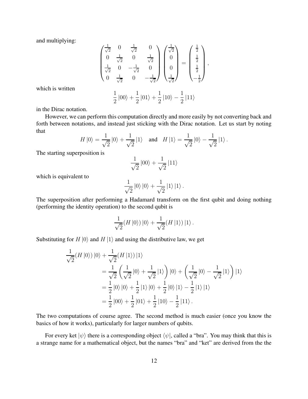
Show extracted searchable text (mathematical glyphs may differ)
and multiplying:
1 1 1 1
√2 0 √2 0 √2 2
1 1 1
0 √2 0 √2 0 2 = , 1 1
√2 0 0 2 √2 0 −1
0 1 0 1 √2 √2 √2 2 −1 −1
which is written
1 1 1
2 |00⟩+ 2 |01⟩+ 2 |10⟩−12 |11⟩
in the Dirac notation.
However, we can perform this computation directly and more easily by not converting back and
forth between notations, and instead just sticking with the Dirac notation. Let us start by noting
that
1 1 1
H and H |0⟩= √ 2 |0⟩+ √ 2 |1⟩ |1⟩= √ 2 |0⟩−1√ 2 |1⟩.
The starting superposition is
1 1
√ 2 |00⟩+ √ 2 |11⟩
which is equivalent to
1 1
√ 2 |0⟩|0⟩+ √ 2 |1⟩|1⟩.
The superposition after performing a Hadamard transform on the first qubit and doing nothing
(performing the identity operation) to the second qubit is
1 1
√ 2 (H |0⟩) |0⟩+ √ 2 (H |1⟩) |1⟩.
HSubstituting for H |0⟩and |1⟩and using the distributive law, we get
1 1
√ 2 (H |0⟩) |0⟩+ √ 2 (H |1⟩) |1⟩
1 1 1 1
= √ 2 √ 2 |0⟩+ √ 2 |1⟩ |0⟩+ √ 2 |0⟩−1√ 2 |1⟩ |1⟩
1 1 1
= 2 |0⟩|0⟩+ 2 |1⟩|0⟩+ 2 |0⟩|1⟩−12 |1⟩|1⟩
1 1 1
= 2 |00⟩+ 2 |01⟩+ 2 |10⟩−12 |11⟩.
The two computations of course agree. The second method is much easier (once you know the
basics of how it works), particularly for larger numbers of qubits.
For every ket |ψ⟩there is a corresponding object ⟨ψ|, called a “bra”. You may think that this isa strange name for a mathematical object, but the names “bra” and “ket” are derived from the the
12
Source page 13
Direct link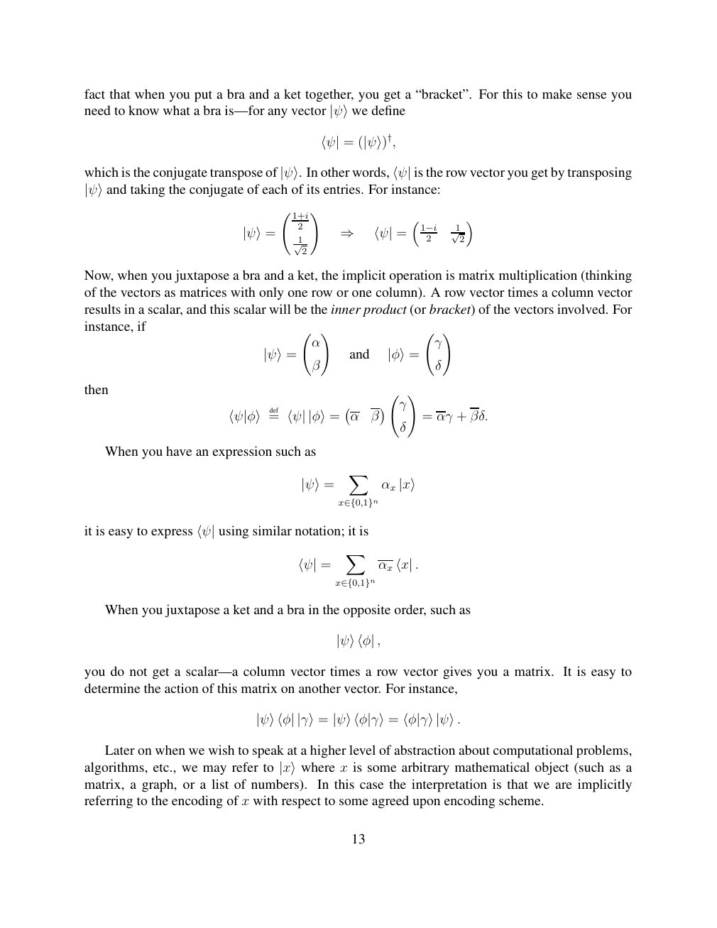
Show extracted searchable text (mathematical glyphs may differ)
fact that when you put a bra and a ket together, you get a “bracket”. For this to make sense you
need to know what a bra is—for any vector |ψ⟩we define
⟨ψ| = (|ψ⟩)†,
which is the conjugate transpose of |ψ⟩. In other words, ⟨ψ| is the row vector you get by transposing
|ψ⟩and taking the conjugate of each of its entries. For instance:
!
1+i
2
1 |ψ⟩= ⇒ ⟨ψ| = 1−i2 √12 √2
Now, when you juxtapose a bra and a ket, the implicit operation is matrix multiplication (thinking
of the vectors as matrices with only one row or one column). A row vector times a column vector
results in a scalar, and this scalar will be the inner product (or bracket) of the vectors involved. For
instance, if ! !
α γ
and |ψ⟩= β |φ⟩= δ
then !
γ
def= α β = αγ + βδ. ⟨ψ|φ⟩ ⟨ψ| |φ⟩= δ
When you have an expression such as
X
|ψ⟩= αx |x⟩
x∈{0,1}n
it is easy to express using similar notation; it is ⟨ψ|
X
⟨ψ| = αx ⟨x| .
x∈{0,1}n
When you juxtapose a ket and a bra in the opposite order, such as
|ψ⟩⟨φ| ,
you do not get a scalar—a column vector times a row vector gives you a matrix. It is easy to
determine the action of this matrix on another vector. For instance,
|ψ⟩⟨φ| |γ⟩= |ψ⟩⟨φ|γ⟩= ⟨φ|γ⟩|ψ⟩.
Later on when we wish to speak at a higher level of abstraction about computational problems,
x is some arbitrary mathematical object (such as aalgorithms, etc., we may refer to |x⟩wherematrix, a graph, or a list of numbers). In this case the interpretation is that we are implicitly
referring to the encoding of x with respect to some agreed upon encoding scheme.
13
⊗ Circuit walkthrough: entanglement and measurement
The Hadamard gate prepares (|0⟩ + |1⟩)/√2 on the first qubit. The controlled-NOT then creates the Bell state (|00⟩ + |11⟩)/√2. Measuring both qubits in the computational basis produces correlated 00 and 11 outcomes, each with ideal probability 1/2. This example illustrates a circuit building block; it is not a complete implementation of the surrounding algorithm.
Show runnable Qiskit example
from qiskit import QuantumCircuit
from qiskit_aer import AerSimulator

qc = QuantumCircuit(2, 2)
qc.h(0)             # Superpose the first qubit
qc.cx(0, 1)         # Entangle both qubits
qc.measure([0, 1], [0, 1])
print(qc.draw(output="text"))
result = AerSimulator().run(qc, shots=1024).result()
print(result.get_counts())  # Approximately 00 and 11
Install qiskit and qiskit-aer locally to execute this code. The diagram is a static circuit illustration, not a browser-based simulator.