Math fidelity: The original PDF page is displayed as a high-resolution image so that equations, bra–ket notation, matrix layouts and circuit diagrams remain exactly as in the source. The expandable text layer is for searching and may not reproduce every mathematical glyph.
Source page 22
Direct link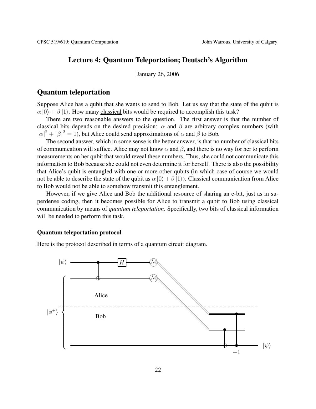
Show extracted searchable text (mathematical glyphs may differ)
CPSC 519/619: Quantum Computation John Watrous, University of Calgary
Lecture 4: Quantum Teleportation; Deutsch’s Algorithm
January 26, 2006
Quantum teleportation
Suppose Alice has a qubit that she wants to send to Bob. Let us say that the state of the qubit is
α β How many classical bits would be required to accomplish this task? |0⟩+ |1⟩. There are two reasonable answers to the question. The first answer is that the number of
classical bits depends on the desired precision: α and β are arbitrary complex numbers (with
α and β to Bob.|α|2 + |β|2 = 1), but Alice could send approximations of The second answer, which in some sense is the better answer, is that no number of classical bits
of communication will suffice. Alice may not know α and β, and there is no way for her to perform
measurements on her qubit that would reveal these numbers. Thus, she could not communicate this
information to Bob because she could not even determine it for herself. There is also the possibility
that Alice’s qubit is entangled with one or more other qubits (in which case of course we would
not be able to describe the state of the qubit as α β Classical communication from Alice |0⟩+ |1⟩).to Bob would not be able to somehow transmit this entanglement.
However, if we give Alice and Bob the additional resource of sharing an e-bit, just as in su-
perdense coding, then it becomes possible for Alice to transmit a qubit to Bob using classical
communication by means of quantum teleportation. Specifically, two bits of classical information
will be needed to perform this task.
Quantum teleportation protocol
Here is the protocol described in terms of a quantum circuit diagram.
|ψ⟩ H M
M Alice
|φ+⟩ Bob
|ψ⟩
−1
22
Source page 23
Direct link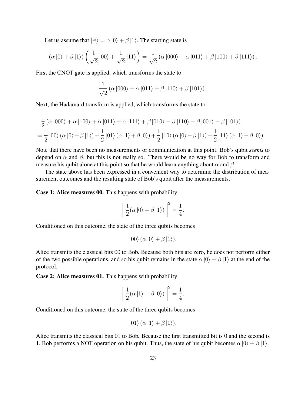
Show extracted searchable text (mathematical glyphs may differ)
Let us assume that α β The starting state is |ψ⟩= |0⟩+ |1⟩.
1 1 1
(α |0⟩+ β |1⟩) √ 2 |00⟩+ √ 2 |11⟩ = √ 2 (α |000⟩+ α |011⟩+ β |100⟩+ β |111⟩) .
First the CNOT gate is applied, which transforms the state to
1
√ 2 (α |000⟩+ α |011⟩+ β |110⟩+ β |101⟩) .
Next, the Hadamard transform is applied, which transforms the state to
1
(α α α α β β 2 |000⟩+ |100⟩+ |011⟩+ |111⟩+ |010⟩−β |110⟩+ |001⟩−β |101⟩)
1 1 1 1
= β + β + + 2 |00⟩(α |0⟩+ |1⟩) 2 |01⟩(α |1⟩+ |0⟩) 2 |10⟩(α |0⟩−β |1⟩) 2 |11⟩(α |1⟩−β |0⟩).
Note that there have been no measurements or communication at this point. Bob’s qubit seems to
depend on α and β, but this is not really so. There would be no way for Bob to transform and
measure his qubit alone at this point so that he would learn anything about α and β.
The state above has been expressed in a convenient way to determine the distribution of mea-
surement outcomes and the resulting state of Bob’s qubit after the measurements.
Case 1: Alice measures 00. This happens with probability
2
1 1
2(α |0⟩+ β |1⟩) = 4.
Conditioned on this outcome, the state of the three qubits becomes
|00⟩(α |0⟩+ β |1⟩).
Alice transmits the classical bits 00 to Bob. Because both bits are zero, he does not perform either
of the two possible operations, and so his qubit remains in the state α β the end of the |0⟩+ |1⟩atprotocol.
Case 2: Alice measures 01. This happens with probability
2
1 1
2(α |1⟩+ β |0⟩) = 4.
Conditioned on this outcome, the state of the three qubits becomes
|01⟩(α |1⟩+ β |0⟩).
Alice transmits the classical bits 01 to Bob. Because the first transmitted bit is 0 and the second is
1, Bob performs a NOT operation on his qubit. Thus, the state of his qubit becomes α β |0⟩+ |1⟩.
23
Source page 24
Direct link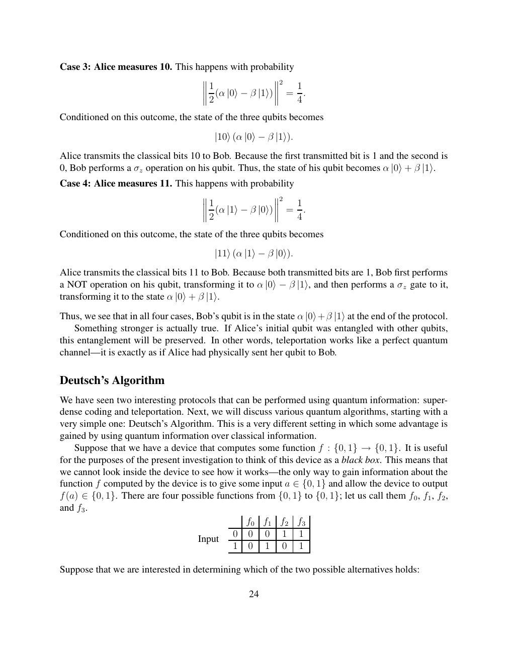
Show extracted searchable text (mathematical glyphs may differ)
Case 3: Alice measures 10. This happens with probability
2
1 1
2(α |0⟩−β |1⟩) = 4.
Conditioned on this outcome, the state of the three qubits becomes
|10⟩(α |0⟩−β |1⟩).
Alice transmits the classical bits 10 to Bob. Because the first transmitted bit is 1 and the second is
0, Bob performs a σz operation on his qubit. Thus, the state of his qubit becomes α β |0⟩+ |1⟩.
Case 4: Alice measures 11. This happens with probability
2
1 1
2(α |1⟩−β |0⟩) = 4.
Conditioned on this outcome, the state of the three qubits becomes
|11⟩(α |1⟩−β |0⟩).
Alice transmits the classical bits 11 to Bob. Because both transmitted bits are 1, Bob first performs
a NOT operation on his qubit, transforming it to α and then performs a σz gate to it, |0⟩−β |1⟩,transforming it to the state α β |0⟩+ |1⟩.
Thus, we see that in all four cases, Bob’s qubit is in the state α the end of the protocol. |0⟩+β |1⟩at Something stronger is actually true. If Alice’s initial qubit was entangled with other qubits,
this entanglement will be preserved. In other words, teleportation works like a perfect quantum
channel—it is exactly as if Alice had physically sent her qubit to Bob.
Deutsch’s Algorithm
We have seen two interesting protocols that can be performed using quantum information: super-
dense coding and teleportation. Next, we will discuss various quantum algorithms, starting with a
very simple one: Deutsch’s Algorithm. This is a very different setting in which some advantage is
gained by using quantum information over classical information.
Suppose that we have a device that computes some function f : It is useful {0, 1} →{0, 1}.for the purposes of the present investigation to think of this device as a black box. This means that
we cannot look inside the device to see how it works—the only way to gain information about the
function f computed by the device is to give some input a and allow the device to output ∈{0, 1}f(a) There are four possible functions from to let us call them f0, f1, f2, ∈{0, 1}. {0, 1} {0, 1};and f3.
f0 f1 f2 f3
Input 0 0 0 1 1
1 0 1 0 1
Suppose that we are interested in determining which of the two possible alternatives holds:
24
Source page 25
Direct link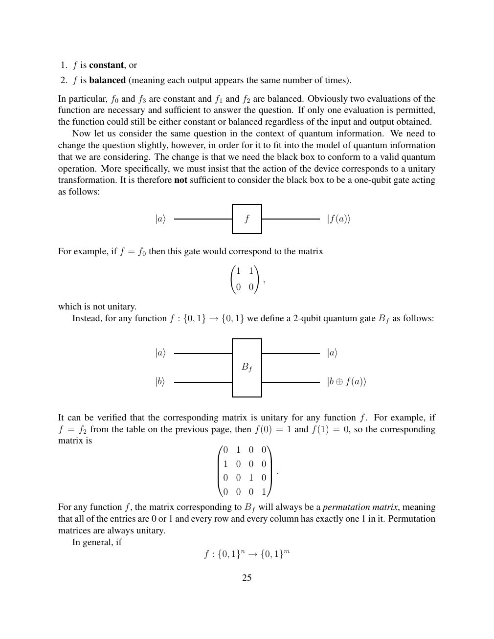
Show extracted searchable text (mathematical glyphs may differ)
1. f is constant, or
2. f is balanced (meaning each output appears the same number of times).
In particular, f0 and f3 are constant and f1 and f2 are balanced. Obviously two evaluations of the
function are necessary and sufficient to answer the question. If only one evaluation is permitted,
the function could still be either constant or balanced regardless of the input and output obtained.
Now let us consider the same question in the context of quantum information. We need to
change the question slightly, however, in order for it to fit into the model of quantum information
that we are considering. The change is that we need the black box to conform to a valid quantum
operation. More specifically, we must insist that the action of the device corresponds to a unitary
transformation. It is therefore not sufficient to consider the black box to be a one-qubit gate acting
as follows:
|a⟩ f |f(a)⟩
For example, if f = f0 then this gate would correspond to the matrix
!
1 1
,
0 0
which is not unitary.
Instead, for any function f : we define a 2-qubit quantum gate Bf as follows: {0, 1} →{0, 1}
|a⟩ |a⟩
Bf
|b⟩ |b ⊕f(a)⟩
It can be verified that the corresponding matrix is unitary for any function f. For example, if
f = f2 from the table on the previous page, then f(0) = 1 and f(1) = 0, so the corresponding
matrix is
0 1 0 0
1 0 0 0
0 0 1 0 .
0 0 0 1
For any function f, the matrix corresponding to Bf will always be a permutation matrix, meaning
that all of the entries are 0 or 1 and every row and every column has exactly one 1 in it. Permutation
matrices are always unitary.
In general, if
f : {0, 1}n →{0, 1}m
25
Source page 26
Direct link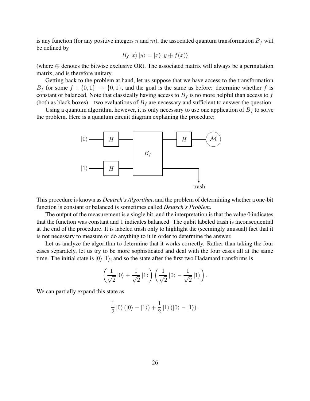
Show extracted searchable text (mathematical glyphs may differ)
is any function (for any positive integers n and m), the associated quantum transformation Bf will
be defined by
Bf |x⟩|y⟩= |x⟩|y ⊕f(x)⟩
(where ⊕denotes the bitwise exclusive OR). The associated matrix will always be a permutationmatrix, and is therefore unitary.
Getting back to the problem at hand, let us suppose that we have access to the transformation
Bf for some f : and the goal is the same as before: determine whether f is {0, 1} →{0, 1},constant or balanced. Note that classically having access to Bf is no more helpful than access to f
(both as black boxes)—two evaluations of Bf are necessary and sufficient to answer the question.
Using a quantum algorithm, however, it is only necessary to use one application of Bf to solve
the problem. Here is a quantum circuit diagram explaining the procedure:
|0⟩ H H M
Bf
|1⟩ H
?
trash
This procedure is known as Deutsch’s Algorithm, and the problem of determining whether a one-bit
function is constant or balanced is sometimes called Deutsch’s Problem.
The output of the measurement is a single bit, and the interpretation is that the value 0 indicates
that the function was constant and 1 indicates balanced. The qubit labeled trash is inconsequential
at the end of the procedure. It is labeled trash only to highlight the (seemingly unusual) fact that it
is not necessary to measure or do anything to it in order to determine the answer.
Let us analyze the algorithm to determine that it works correctly. Rather than taking the four
cases separately, let us try to be more sophisticated and deal with the four cases all at the same
time. The initial state is |0⟩|1⟩, and so the state after the first two Hadamard transforms is
1 1 1
. √ 2 |0⟩+ √ 2 |1⟩ √ 2 |0⟩−1√ 2 |1⟩
We can partially expand this state as
1 1
+ . 2 |0⟩(|0⟩−|1⟩) 2 |1⟩(|0⟩−|1⟩)
26
Source page 27
Direct link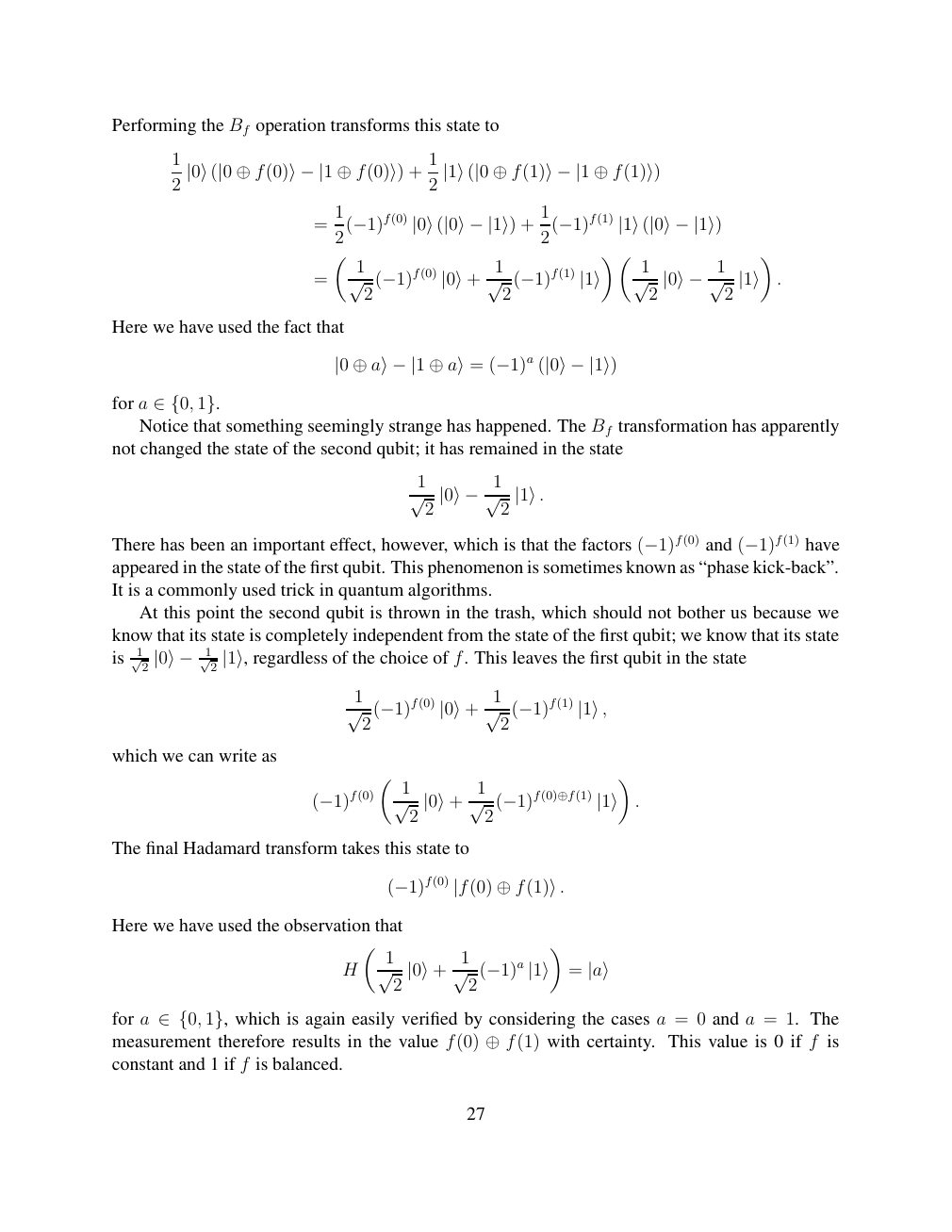
Show extracted searchable text (mathematical glyphs may differ)
Performing the Bf operation transforms this state to
1 1
+ 2 |0⟩(|0 ⊕f(0)⟩−|1 ⊕f(0)⟩) 2 |1⟩(|0 ⊕f(1)⟩−|1 ⊕f(1)⟩)
1 1
= 2(−1)f(0) |0⟩(|0⟩−|1⟩) + 2(−1)f(1) |1⟩(|0⟩−|1⟩)
1 1 1
. = √ 2(−1)f(0) |0⟩+ √ 2(−1)f(1) |1⟩ √ 2 |0⟩−1√ 2 |1⟩
Here we have used the fact that
|0 ⊕a⟩−|1 ⊕a⟩= (−1)a (|0⟩−|1⟩)
for a ∈{0, 1}. Notice that something seemingly strange has happened. The Bf transformation has apparently
not changed the state of the second qubit; it has remained in the state
1
√ 2 |0⟩−1√ 2 |1⟩.
There has been an important effect, however, which is that the factors (−1)f(0) and (−1)f(1) haveappeared in the state of the first qubit. This phenomenon is sometimes known as “phase kick-back”.
It is a commonly used trick in quantum algorithms.
At this point the second qubit is thrown in the trash, which should not bother us because we
know that its state is completely independent from the state of the first qubit; we know that its state
is √12 √12 regardless of the choice of f. This leaves the first qubit in the state |0⟩− |1⟩,
1 1
√ 2 (−1)f(0) |0⟩+ √ 2 (−1)f(1) |1⟩,
which we can write as
1 1
(−1)f(0) √ 2 |0⟩+ √ 2 (−1)f(0)⊕f(1) |1⟩ .
The final Hadamard transform takes this state to
(−1)f(0) |f(0) ⊕f(1)⟩.
Here we have used the observation that
1 1
H √ 2 |0⟩+ √ 2 (−1)a |1⟩ = |a⟩
for a which is again easily verified by considering the cases a = 0 and a = 1. The ∈{0, 1},measurement therefore results in the value f(0) with certainty. This value is 0 if f is ⊕f(1)constant and 1 if f is balanced.
27
⊗ Circuit walkthrough: entanglement and measurement
The Hadamard gate prepares (|0⟩ + |1⟩)/√2 on the first qubit. The controlled-NOT then creates the Bell state (|00⟩ + |11⟩)/√2. Measuring both qubits in the computational basis produces correlated 00 and 11 outcomes, each with ideal probability 1/2. This example illustrates a circuit building block; it is not a complete implementation of the surrounding algorithm.
Show runnable Qiskit example
from qiskit import QuantumCircuit
from qiskit_aer import AerSimulator

qc = QuantumCircuit(2, 2)
qc.h(0)             # Superpose the first qubit
qc.cx(0, 1)         # Entangle both qubits
qc.measure([0, 1], [0, 1])
print(qc.draw(output="text"))
result = AerSimulator().run(qc, shots=1024).result()
print(result.get_counts())  # Approximately 00 and 11
Install qiskit and qiskit-aer locally to execute this code. The diagram is a static circuit illustration, not a browser-based simulator.