Math fidelity: The original PDF page is displayed as a high-resolution image so that equations, bra–ket notation, matrix layouts and circuit diagrams remain exactly as in the source. The expandable text layer is for searching and may not reproduce every mathematical glyph.
Source page 48
Direct link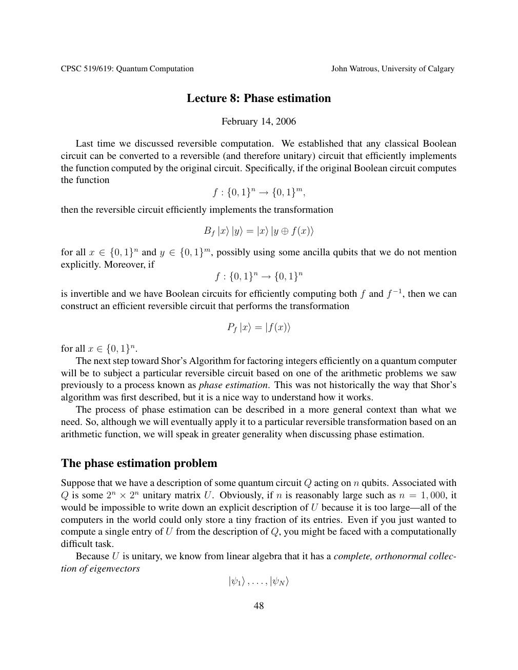
Show extracted searchable text (mathematical glyphs may differ)
CPSC 519/619: Quantum Computation John Watrous, University of Calgary
Lecture 8: Phase estimation
February 14, 2006
Last time we discussed reversible computation. We established that any classical Boolean
circuit can be converted to a reversible (and therefore unitary) circuit that efficiently implements
the function computed by the original circuit. Specifically, if the original Boolean circuit computes
the function
f : {0, 1}n →{0, 1}m,
then the reversible circuit efficiently implements the transformation
Bf |x⟩|y⟩= |x⟩|y ⊕f(x)⟩
for all x and y possibly using some ancilla qubits that we do not mention ∈{0, 1}n ∈{0, 1}m,explicitly. Moreover, if
f : {0, 1}n →{0, 1}n
is invertible and we have Boolean circuits for efficiently computing both f and f −1, then we can
construct an efficient reversible circuit that performs the transformation
Pf |x⟩= |f(x)⟩
for all x ∈{0, 1}n. The next step toward Shor’s Algorithm for factoring integers efficiently on a quantum computer
will be to subject a particular reversible circuit based on one of the arithmetic problems we saw
previously to a process known as phase estimation. This was not historically the way that Shor’s
algorithm was first described, but it is a nice way to understand how it works.
The process of phase estimation can be described in a more general context than what we
need. So, although we will eventually apply it to a particular reversible transformation based on an
arithmetic function, we will speak in greater generality when discussing phase estimation.
The phase estimation problem
Suppose that we have a description of some quantum circuit Q acting on n qubits. Associated with
Q is some 2n 2n unitary matrix U. Obviously, if n is reasonably large such as n = 1, 000, it ×would be impossible to write down an explicit description of U because it is too large—all of the
computers in the world could only store a tiny fraction of its entries. Even if you just wanted to
compute a single entry of U from the description of Q, you might be faced with a computationally
difficult task.
Because U is unitary, we know from linear algebra that it has a complete, orthonormal collec-
tion of eigenvectors
|ψ1⟩, . . . , |ψN⟩
48
Source page 49
Direct link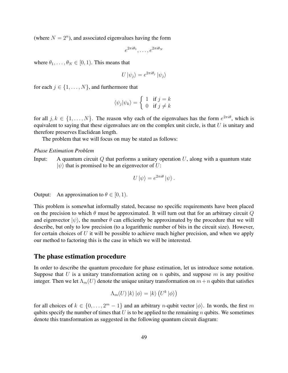
Show extracted searchable text (mathematical glyphs may differ)
(where N = 2n), and associated eigenvalues having the form
e2πiθ1, . . . , e2πiθN
where θ1, . . . , θN 1). This means that ∈[0,
U |ψj⟩= e2πiθj |ψj⟩
for each j . . . , and furthermore that ∈{1, N},
1 if j = k
⟨ψj|ψk⟩= 0 if j k ̸=
for all j, k . . . , The reason why each of the eigenvalues has the form e2πiθ, which is ∈{1, N}.equivalent to saying that these eigenvalues are on the complex unit circle, is that U is unitary and
therefore preserves Euclidean length.
The problem that we will focus on may be stated as follows:
Phase Estimation Problem
Input: A quantum circuit Q that performs a unitary operation U, along with a quantum state
|ψ⟩that is promised to be an eigenvector of U:
U |ψ⟩= e2πiθ |ψ⟩.
Output: An approximation to θ 1). ∈[0,
This problem is somewhat informally stated, because no specific requirements have been placed
on the precision to which θ must be approximated. It will turn out that for an arbitrary circuit Q
θ can efficiently be approximated by the procedure that we willand eigenvector |ψ⟩, the numberdescribe, but only to low precision (to a logarithmic number of bits in the circuit size). However,
for certain choices of U it will be possible to achieve much higher precision, and when we apply
our method to factoring this is the case in which we will be interested.
The phase estimation procedure
In order to describe the quantum procedure for phase estimation, let us introduce some notation.
Suppose that U is a unitary transformation acting on n qubits, and suppose m is any positive
integer. Then we let Λm(U) denote the unique unitary transformation on m+n qubits that satisfies
Λm(U) |k⟩|φ⟩= |k⟩ U k |φ⟩
for all choices of k . . . , 2m and an arbitrary n-qubit vector In words, the first m ∈{0, −1} |φ⟩.qubits specify the number of times that U is to be applied to the remaining n qubits. We sometimes
denote this transformation as suggested in the following quantum circuit diagram:
49
Source page 50
Direct link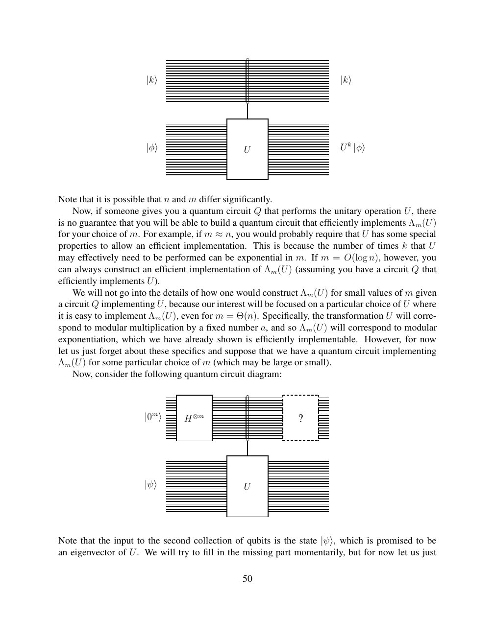
Show extracted searchable text (mathematical glyphs may differ)
|k⟩ |k⟩
U k U |φ⟩ |φ⟩
Note that it is possible that n and m differ significantly.
Now, if someone gives you a quantum circuit Q that performs the unitary operation U, there
is no guarantee that you will be able to build a quantum circuit that efficiently implements Λm(U)
U has some specialfor your choice of m. For example, if m ≈n, you would probably require thatproperties to allow an efficient implementation. This is because the number of times k that U
may effectively need to be performed can be exponential in m. If m = O(log n), however, you
can always construct an efficient implementation of Λm(U) (assuming you have a circuit Q that
efficiently implements U).
We will not go into the details of how one would construct Λm(U) for small values of m given
a circuit Q implementing U, because our interest will be focused on a particular choice of U where
it is easy to implement Λm(U), even for m = Θ(n). Specifically, the transformation U will corre-
spond to modular multiplication by a fixed number a, and so Λm(U) will correspond to modular
exponentiation, which we have already shown is efficiently implementable. However, for now
let us just forget about these specifics and suppose that we have a quantum circuit implementing
Λm(U) for some particular choice of m (which may be large or small).
Now, consider the following quantum circuit diagram:
|0m⟩ H⊗m ?
U |ψ⟩
Note that the input to the second collection of qubits is the state |ψ⟩, which is promised to bean eigenvector of U. We will try to fill in the missing part momentarily, but for now let us just
50
Source page 51
Direct link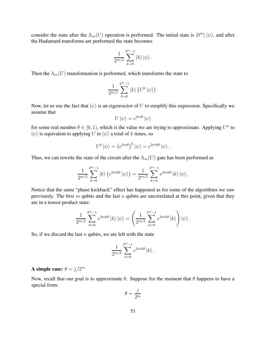
Show extracted searchable text (mathematical glyphs may differ)
consider the state after the Λm(U) operation is performed. The initial state is |0m⟩|ψ⟩, and afterthe Hadamard transforms are performed the state becomes
1 2m−1X
2m/2 |k⟩|ψ⟩.
k=0
Then the Λm(U) transformation is performed, which transforms the state to
1 2m−1X k U . 2m/2 |k⟩ |ψ⟩
k=0
U to simplify this expression. Specifically weNow, let us use the fact that |ψ⟩is an eigenvector ofassume that
U |ψ⟩= e2πiθ |ψ⟩
for some real number θ 1), which is the value we are trying to approximate. Applying U k to ∈[0, k times, so|ψ⟩is equivalent to applying U to |ψ⟩a total of
k k
U |ψ⟩= e2πiθ |ψ⟩= e2πikθ |ψ⟩.
Thus, we can rewrite the state of the circuit after the Λm(U) gate has been performed as
1 2m−1X 1 2m−1X
e2πikθ = e2πikθ 2m/2 |k⟩ |ψ⟩ 2m/2 |k⟩|ψ⟩.
k=0 k=0
Notice that the same “phase kickback” effect has happened as for some of the algorithms we saw
previously. The first m qubits and the last n qubits are uncorrelated at this point, given that they
are in a tensor product state:
!
1 2m−1X 1 2m−1X
e2πikθ e2πikθ 2m/2 |k⟩|ψ⟩= 2m/2 |k⟩ |ψ⟩.
k=0 k=0
So, if we discard the last n qubits, we are left with the state
1 2m−1X
e2πikθ 2m/2 |k⟩.
k=0
A simple case: θ = j/2m
Now, recall that our goal is to approximate θ. Suppose for the moment that θ happens to have a
special form:
j
θ =
2m
51
Source page 52
Direct link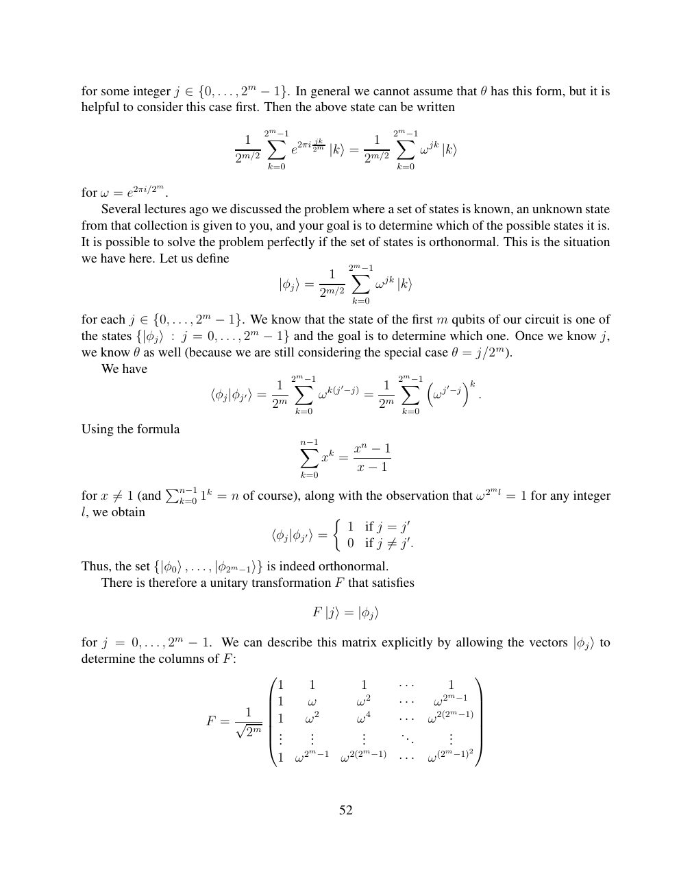
Show extracted searchable text (mathematical glyphs may differ)
for some integer j . . . , 2m In general we cannot assume that θ has this form, but it is ∈{0, −1}.helpful to consider this case first. Then the above state can be written
1 2m−1X jk 1 2m−1X
e2πi 2m ωjk 2m/2 |k⟩= 2m/2 |k⟩
k=0 k=0
for ω = e2πi/2m.
Several lectures ago we discussed the problem where a set of states is known, an unknown state
from that collection is given to you, and your goal is to determine which of the possible states it is.
It is possible to solve the problem perfectly if the set of states is orthonormal. This is the situation
we have here. Let us define
1 2m−1X
|φj⟩= 2m/2 ωjk |k⟩
k=0
for each j . . . , 2m We know that the state of the first m qubits of our circuit is one of ∈{0, −1}.the states j = 0, . . . , 2m and the goal is to determine which one. Once we know j, {|φj⟩: −1}we know θ as well (because we are still considering the special case θ = j/2m).
We have
1 2m−1X 1 2m−1X ωk(j′−j) = ωj′−j k . ⟨φj|φj′⟩= 2m 2m
k=0 k=0
Using the formula
Xn−1 xn xk = −1
x
k=0 −1
for x 1 (and Pn−1k=0 1k = n of course), along with the observation that ω2ml = 1 for any integer ̸=l, we obtain
1 if j = j′
⟨φj|φj′⟩= 0 if j j′. ̸=
Thus, the set . . . , is indeed orthonormal. {|φ0⟩, |φ2m−1⟩} There is therefore a unitary transformation F that satisfies
F |j⟩= |φj⟩
for j = 0, . . . , 2m −1. We can describe this matrix explicitly by allowing the vectors |φj⟩todetermine the columns of F:
1 1 1 · · · 1 1 ω ω2 ω2m−1 1 · · ·
F = √ 2m 1 ω2 ω4 · · · ω2(2m−1) ... ... ... ... ...
1 ω2m−1 ω2(2m−1) ω(2m−1)2 · · ·
52
Source page 53
Direct link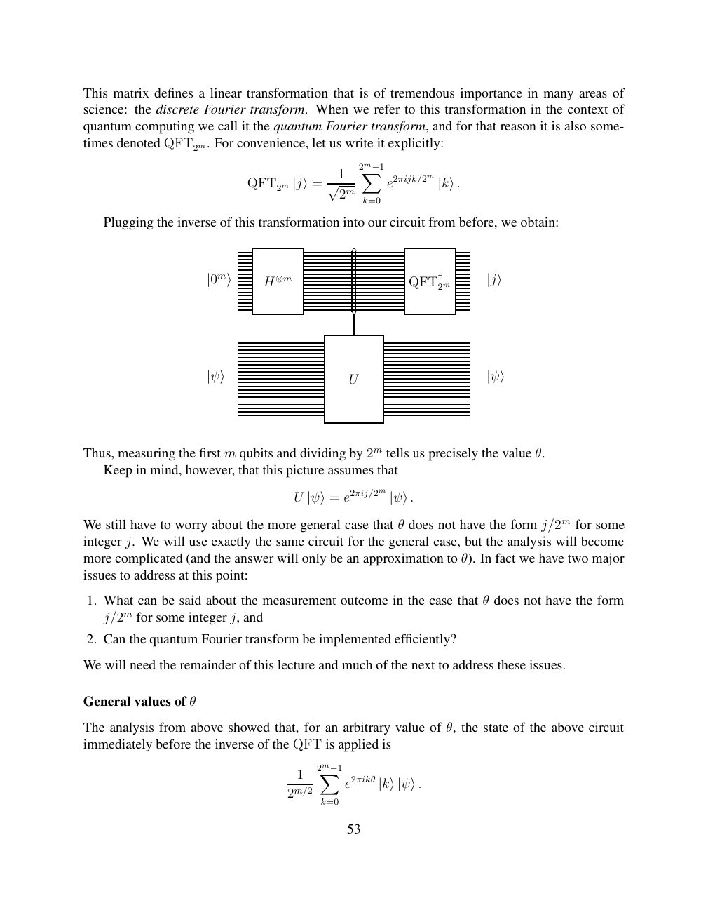
Show extracted searchable text (mathematical glyphs may differ)
This matrix defines a linear transformation that is of tremendous importance in many areas of
science: the discrete Fourier transform. When we refer to this transformation in the context of
quantum computing we call it the quantum Fourier transform, and for that reason it is also some-
times denoted QFT2m. For convenience, let us write it explicitly:
1 2m−1X
QFT2m |j⟩= √ 2m e2πijk/2m |k⟩. k=0
Plugging the inverse of this transformation into our circuit from before, we obtain:
2m |0m⟩ H⊗m QFT† |j⟩
U |ψ⟩ |ψ⟩
Thus, measuring the first m qubits and dividing by 2m tells us precisely the value θ.
Keep in mind, however, that this picture assumes that
U e2πij/2m |ψ⟩= |ψ⟩.
We still have to worry about the more general case that θ does not have the form j/2m for some
integer j. We will use exactly the same circuit for the general case, but the analysis will become
more complicated (and the answer will only be an approximation to θ). In fact we have two major
issues to address at this point:
1. What can be said about the measurement outcome in the case that θ does not have the form
j/2m for some integer j, and
2. Can the quantum Fourier transform be implemented efficiently?
We will need the remainder of this lecture and much of the next to address these issues.
General values of θ
The analysis from above showed that, for an arbitrary value of θ, the state of the above circuit
immediately before the inverse of the QFT is applied is
1 2m−1X
e2πikθ 2m/2 |k⟩|ψ⟩.
k=0
53
Source page 54
Direct link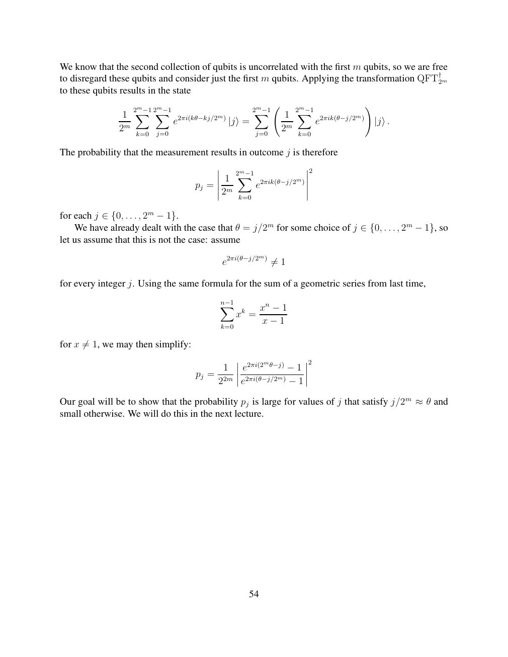
Show extracted searchable text (mathematical glyphs may differ)
We know that the second collection of qubits is uncorrelated with the first m qubits, so we are free
to disregard these qubits and consider just the first m qubits. Applying the transformation QFT†2m
to these qubits results in the state
!
1 2m−1X 2m−1X 2m−1X 1 2m−1X
e2πi(kθ−kj/2m) e2πik(θ−j/2m) 2m |j⟩= 2m |j⟩.
k=0 j=0 j=0 k=0
The probability that the measurement results in outcome j is therefore
2
1 2m−1X
pj = e2πik(θ−j/2m)
2m
k=0
for each j . . . , 2m ∈{0, −1}. We have already dealt with the case that θ = j/2m for some choice of j . . . , 2m so ∈{0, −1},let us assume that this is not the case: assume
e2πi(θ−j/2m) 1 ̸=
for every integer j. Using the same formula for the sum of a geometric series from last time,
Xn−1 xn xk = −1
x
k=0 −1
for x 1, we may then simplify: ̸=
2
1 e2πi(2mθ−j) pj = −1
22m e2πi(θ−j/2m) −1
Our goal will be to show that the probability pj is large for values of j that satisfy j/2m and ≈θsmall otherwise. We will do this in the next lecture.
54
⊗ Circuit walkthrough: entanglement and measurement
The Hadamard gate prepares (|0⟩ + |1⟩)/√2 on the first qubit. The controlled-NOT then creates the Bell state (|00⟩ + |11⟩)/√2. Measuring both qubits in the computational basis produces correlated 00 and 11 outcomes, each with ideal probability 1/2. This example illustrates a circuit building block; it is not a complete implementation of the surrounding algorithm.
Show runnable Qiskit example
from qiskit import QuantumCircuit
from qiskit_aer import AerSimulator

qc = QuantumCircuit(2, 2)
qc.h(0)             # Superpose the first qubit
qc.cx(0, 1)         # Entangle both qubits
qc.measure([0, 1], [0, 1])
print(qc.draw(output="text"))
result = AerSimulator().run(qc, shots=1024).result()
print(result.get_counts())  # Approximately 00 and 11
Install qiskit and qiskit-aer locally to execute this code. The diagram is a static circuit illustration, not a browser-based simulator.