Math fidelity: The original PDF page is displayed as a high-resolution image so that equations, bra–ket notation, matrix layouts and circuit diagrams remain exactly as in the source. The expandable text layer is for searching and may not reproduce every mathematical glyph.
Source page 55
Direct link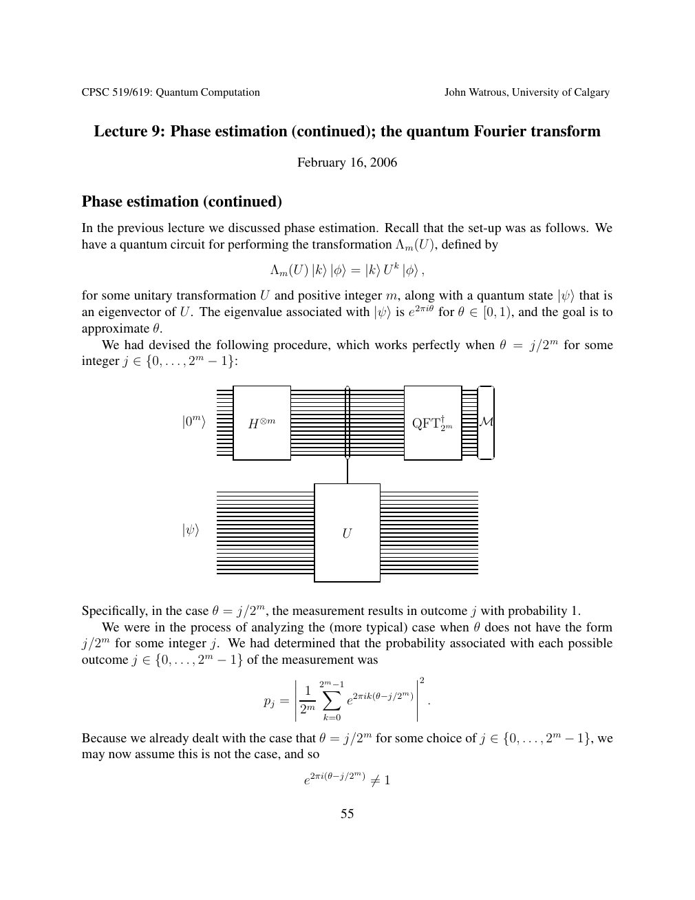
Show extracted searchable text (mathematical glyphs may differ)
CPSC 519/619: Quantum Computation John Watrous, University of Calgary
Lecture 9: Phase estimation (continued); the quantum Fourier transform
February 16, 2006
Phase estimation (continued)
In the previous lecture we discussed phase estimation. Recall that the set-up was as follows. We
have a quantum circuit for performing the transformation Λm(U), defined by
Λm(U) |k⟩|φ⟩= |k⟩U k |φ⟩,
for some unitary transformation U and positive integer m, along with a quantum state |ψ⟩that is 1), and the goal is toan eigenvector of U. The eigenvalue associated with |ψ⟩is e2πiθ for θ ∈[0,approximate θ.
We had devised the following procedure, which works perfectly when θ = j/2m for some
integer j . . . , 2m ∈{0, −1}:
2m M |0m⟩ H⊗m QFT†
U |ψ⟩
Specifically, in the case θ = j/2m, the measurement results in outcome j with probability 1.
We were in the process of analyzing the (more typical) case when θ does not have the form
j/2m for some integer j. We had determined that the probability associated with each possible
outcome j . . . , 2m of the measurement was ∈{0, −1}
2
1 2m−1X
pj = e2πik(θ−j/2m) .
2m
k=0
Because we already dealt with the case that θ = j/2m for some choice of j . . . , 2m we ∈{0, −1},may now assume this is not the case, and so
e2πi(θ−j/2m) 1 ̸=
55
Source page 56
Direct link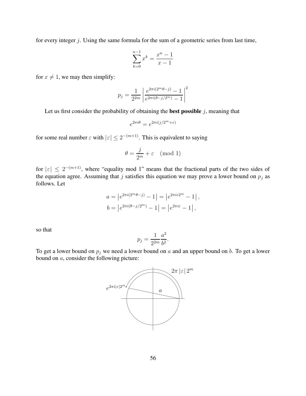
Show extracted searchable text (mathematical glyphs may differ)
for every integer j. Using the same formula for the sum of a geometric series from last time,
Xn−1 xn xk = −1
x
k=0 −1
for x 1, we may then simplify: ̸=
2
1 e2πi(2mθ−j) pj = −1
22m e2πi(θ−j/2m) −1
Let us first consider the probability of obtaining the best possible j, meaning that
e2πiθ = e2πi(j/2m+ε)
for some real number ε with This is equivalent to saying |ε| ≤2−(m+1).
j
θ = + ε (mod 1)
2m
for where “equality mod 1” means that the fractional parts of the two sides of |ε| ≤2−(m+1),the equation agree. Assuming that j satisfies this equation we may prove a lower bound on pj as
follows. Let
a = e2πi(2mθ−j) = e2πiε2m , −1 −1
b = e2πi(θ−j/2m) = e2πiε , −1 −1
so that
1 a2
pj = .
22m b2
To get a lower bound on pj we need a lower bound on a and an upper bound on b. To get a lower
bound on a, consider the following picture:
2π |ε| 2m
e2πi|ε|2m a
56
Source page 57
Direct link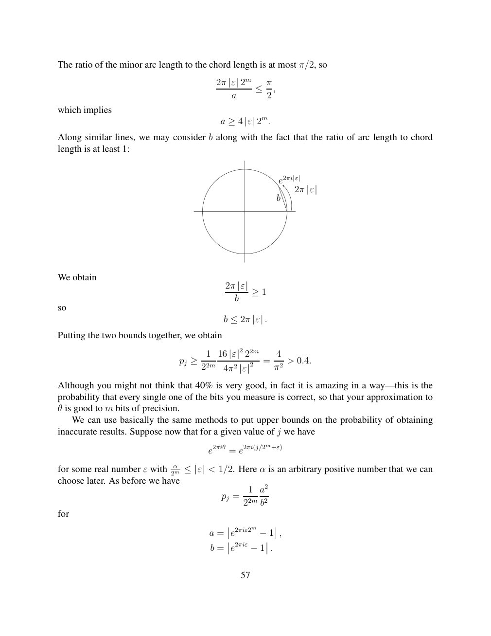
Show extracted searchable text (mathematical glyphs may differ)
The ratio of the minor arc length to the chord length is at most π/2, so
2π |ε| 2m a ≤π2,
which implies
a ≥4 |ε| 2m.
Along similar lines, we may consider b along with the fact that the ratio of arc length to chord
length is at least 1:
e2πi|ε|
2π |ε| b
We obtain
2π |ε| b ≥1
so
b ≤2π |ε| .
Putting the two bounds together, we obtain
1 16 22m 4 pj |ε|2 = > 0.4. ≥ 22m 4π2 π2 |ε|2
Although you might not think that 40% is very good, in fact it is amazing in a way—this is the
probability that every single one of the bits you measure is correct, so that your approximation to
θ is good to m bits of precision.
We can use basically the same methods to put upper bounds on the probability of obtaining
inaccurate results. Suppose now that for a given value of j we have
e2πiθ = e2πi(j/2m+ε)
< 1/2. Here α is an arbitrary positive number that we canfor some real number ε with 2mα ≤|ε|choose later. As before we have
1 a2
pj =
22m b2
for
a = e2πiε2m , −1
b = e2πiε −1 .
57
Source page 58
Direct link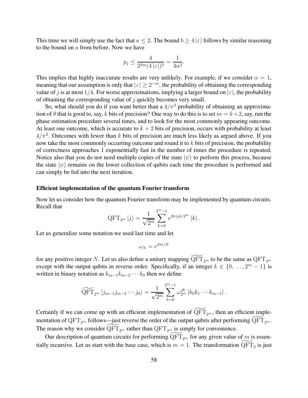
Show extracted searchable text (mathematical glyphs may differ)
follows by similar reasoningThis time we will simply use the fact that a ≤2. The bound b ≥4 |ε|to the bound on a from before. Now we have
4 1
pj ≤ 22m(4 = 4α2. |ε|)2
This implies that highly inaccurate results are very unlikely. For example, if we consider α = 1,
meaning that our assumption is only that the probability of obtaining the corresponding |ε| ≥2−m,
value of j is at most 1/4. For worse approximations, implying a larger bound on |ε|, the probabilityof obtaining the corresponding value of j quickly becomes very small.
So, what should you do if you want better than a 4/π2 probability of obtaining an approxima-
tion of θ that is good to, say, k bits of precision? One way to do this is to set m = k+2, say, run the
phase estimation procedure several times, and to look for the most commonly appearing outcome.
At least one outcome, which is accurate to k + 2 bits of precision, occurs with probability at least
4/π2. Outcomes with fewer than k bits of precision are much less likely as argued above. If you
now take the most commonly occurring outcome and round it to k bits of precision, the probability
of correctness approaches 1 exponentially fast in the number of times the procedure is repeated.
Notice also that you do not need multiple copies of the state |ψ⟩to perform this process, because
the state |ψ⟩remains on the lower collection of qubits each time the procedure is performed andcan simply be fed into the next iteration.
Efficient implementation of the quantum Fourier transform
Now let us consider how the quantum Fourier transform may be implemented by quantum circuits.
Recall that
1 2m−1X
QFT2m |j⟩= √ 2m e2πijk/2m |k⟩. k=0
Let us generalize some notation we used last time and let
ωN = e2πi/N
for any positive integer N. Let us also define a unitary mapping QFT2m] to be the same as QFT2m
except with the output qubits in reverse order. Specifically, if an integer k . . . , 2m is ∈{0, −1}written in binary notation as k0 then we define km−1km−2 · · ·
1 2m−1X
QFT2m ] ωjk2m |jm−1jm−2 · · · j0⟩= √ 2m |k0k1 · · · km−1⟩. k=0
Certainly if we can come up with an efficient implementation of QFT2m,] then an efficient imple-
mentation of QFT2m follows—just reverse the order of the output qubits after performing QFT2m.]
The reason why we consider QFT2m] rather than QFT2m is simply for convenience.
Our description of quantum circuits for performing QFT2m] for any given value of m is essen-
tially recursive. Let us start with the base case, which is m = 1. The transformation QFT2] is just
58
Source page 59
Direct link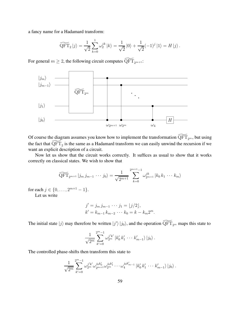
Show extracted searchable text (mathematical glyphs may differ)
a fancy name for a Hadamard transform:
X1 1 1 1
QFT2 ] ωjk2 H |j⟩= √ 2 |k⟩= √ 2 |0⟩+ √ 2(−1)j |1⟩= |j⟩. k=0
For general m ≥2, the following circuit computes QFT2m+1:]
|jm⟩
|jm−1⟩
] QFT2m
|j1⟩
|j0⟩ H ω2m+1 ω2m ω4
Of course the diagram assumes you know how to implement the transformation QFT2m,] but using
the fact that QFT2] is the same as a Hadamard transform we can easily unwind the recursion if we
want an explicit description of a circuit.
Now let us show that the circuit works correctly. It suffices as usual to show that it works
correctly on classical states. We wish to show that
1 2m+1−1X
QFT2m+1 ] ωjk2m+1 k1 |jm jm−1 · · · j0⟩= √ 2m+1 |k0 · · · km⟩ k=0
for each j . . . , 2m+1 ∈{0, −1}. Let us write
j′ = jm jm−1 · · · j1 = ⌊j/2⌋,
k′ = km−1 km−2 · · · k0 = k −km2m.
] maps this state to QFT2mThe initial state |j⟩may therefore be written |j′⟩|j0⟩, and the operation
1 2m−1X
ωj′k′2m 0 k′1 k′ √ 2m |k′ · · · m−1⟩|j0⟩. k′=0
The controlled phase-shifts then transform this state to
1 2m−1X j0k′0 j0k′1 j0k′m−1 ωj′k′2m ω 2m+1ω 2m ω 4 0 k′1 k′ √ 2m · · · |k′ · · · m−1⟩|j0⟩. k′=0
59
Source page 60
Direct link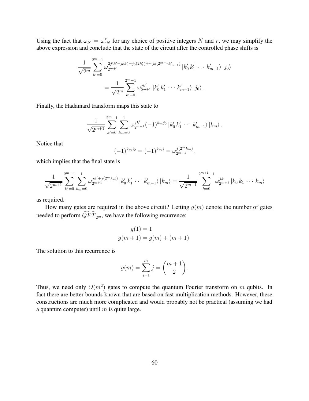
Show extracted searchable text (mathematical glyphs may differ)
Using the fact that ωN = ωrrN for any choice of positive integers N and r, we may simplify the
above expression and conclude that the state of the circuit after the controlled phase shifts is
1 2m−1X 2j′k′+j0k′0+j0(2k′ m−1) 1)+···j0(2m−1k′ ω 2m+1 √ 2m |k′0 k′1 · · · k′m−1⟩|j0⟩ k′=0
1 2m−1X
= ωjk′2m+1 0 k′1 k′ √ 2m |k′ · · · m−1⟩|j0⟩. k′=0
Finally, the Hadamard transform maps this state to
1 2m−1X X1
ωjk′ 0 k′1 k′ √ 2m+1 2m+1(−1)kmj0 |k′ · · · m−1⟩|km⟩. k′=0 km=0
Notice that
2m+1 , (−1)kmj0 = (−1)kmj = ωj(2mkm)
which implies that the final state is
1 2m−1X X1 1 2m+1−1X
ωjk′+j(2mkm)2m+1 0 k′1 k′ ωjk2m+1 k1 √2m+1 |k′ · · · m−1⟩|km⟩= √ 2m+1 |k0 · · · km⟩ k′=0 km=0 k=0
as required.
How many gates are required in the above circuit? Letting g(m) denote the number of gates
needed to perform QFT] 2m, we have the following recurrence:
g(1) = 1
g(m + 1) = g(m) + (m + 1).
The solution to this recurrence is
Xm m + 1
g(m) = j = .
2
j=1
Thus, we need only O(m2) gates to compute the quantum Fourier transform on m qubits. In
fact there are better bounds known that are based on fast multiplication methods. However, these
constructions are much more complicated and would probably not be practical (assuming we had
a quantum computer) until m is quite large.
60
⊗ Circuit walkthrough: entanglement and measurement
The Hadamard gate prepares (|0⟩ + |1⟩)/√2 on the first qubit. The controlled-NOT then creates the Bell state (|00⟩ + |11⟩)/√2. Measuring both qubits in the computational basis produces correlated 00 and 11 outcomes, each with ideal probability 1/2. This example illustrates a circuit building block; it is not a complete implementation of the surrounding algorithm.
Show runnable Qiskit example
from qiskit import QuantumCircuit
from qiskit_aer import AerSimulator

qc = QuantumCircuit(2, 2)
qc.h(0)             # Superpose the first qubit
qc.cx(0, 1)         # Entangle both qubits
qc.measure([0, 1], [0, 1])
print(qc.draw(output="text"))
result = AerSimulator().run(qc, shots=1024).result()
print(result.get_counts())  # Approximately 00 and 11
Install qiskit and qiskit-aer locally to execute this code. The diagram is a static circuit illustration, not a browser-based simulator.