Math fidelity: The original PDF page is displayed as a high-resolution image so that equations, bra–ket notation, matrix layouts and circuit diagrams remain exactly as in the source. The expandable text layer is for searching and may not reproduce every mathematical glyph.
Source page 88
Direct link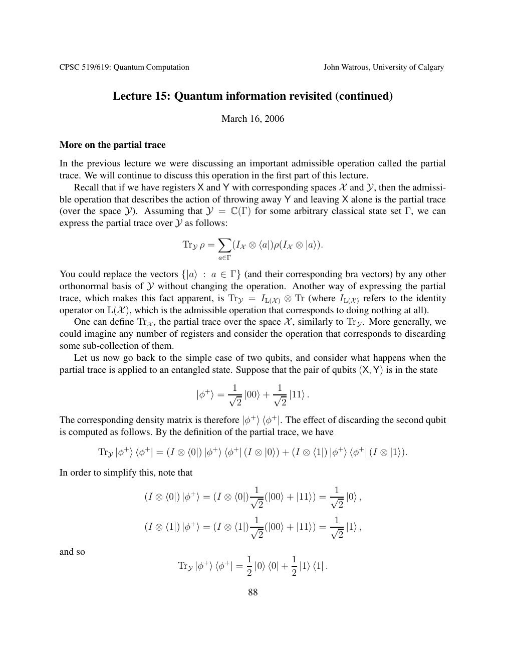
Show extracted searchable text (mathematical glyphs may differ)
CPSC 519/619: Quantum Computation John Watrous, University of Calgary
Lecture 15: Quantum information revisited (continued)
March 16, 2006
More on the partial trace
In the previous lecture we were discussing an important admissible operation called the partial
trace. We will continue to discuss this operation in the first part of this lecture.
Recall that if we have registers X and Y with corresponding spaces and then the admissi- Y XX Y,ble operation that describes the action of throwing away and leaving alone is the partial trace
= C(Γ) for some arbitrary classical state set Γ, we can(over the space Y). Assuming that Yexpress the partial trace over as follows: Y X
TrY ρ = (IX ⊗⟨a|)ρ(IX ⊗|a⟩).
a∈Γ
You could replace the vectors a (and their corresponding bra vectors) by any other {|a⟩: ∈Γ}orthonormal basis of without changing the operation. Another way of expressing the partial Ytrace, which makes this fact apparent, is = ) (where ) refers to the identity TrY IL(X ⊗Tr IL(Xoperator on ), which is the admissible operation that corresponds to doing nothing at all). L(X
One can define TrX, the partial trace over the space X , similarly to TrY. More generally, wecould imagine any number of registers and consider the operation that corresponds to discarding
some sub-collection of them.
Let us now go back to the simple case of two qubits, and consider what happens when the
partial trace is applied to an entangled state. Suppose that the pair of qubits (X, Y) is in the state
1 1
|φ+⟩= √ 2 |00⟩+ √ 2 |11⟩.
The corresponding density matrix is therefore |φ+⟩⟨φ+|. The effect of discarding the second qubitis computed as follows. By the definition of the partial trace, we have
TrY |φ+⟩⟨φ+| = (I ⊗⟨0|) |φ+⟩⟨φ+| (I ⊗|0⟩) + (I ⊗⟨1|) |φ+⟩⟨φ+| (I ⊗|1⟩).
In order to simplify this, note that
1 1
(I ⊗⟨0|) |φ+⟩= (I ⊗⟨0|) √ 2(|00⟩+ |11⟩) = √ 2 |0⟩,
1 1
(I ⊗⟨1|) |φ+⟩= (I ⊗⟨1|) √ 2(|00⟩+ |11⟩) = √ 2 |1⟩,
and so
1 1
TrY |φ+⟩⟨φ+| = 2 |0⟩⟨0| + 2 |1⟩⟨1| .
88
Source page 89
Direct link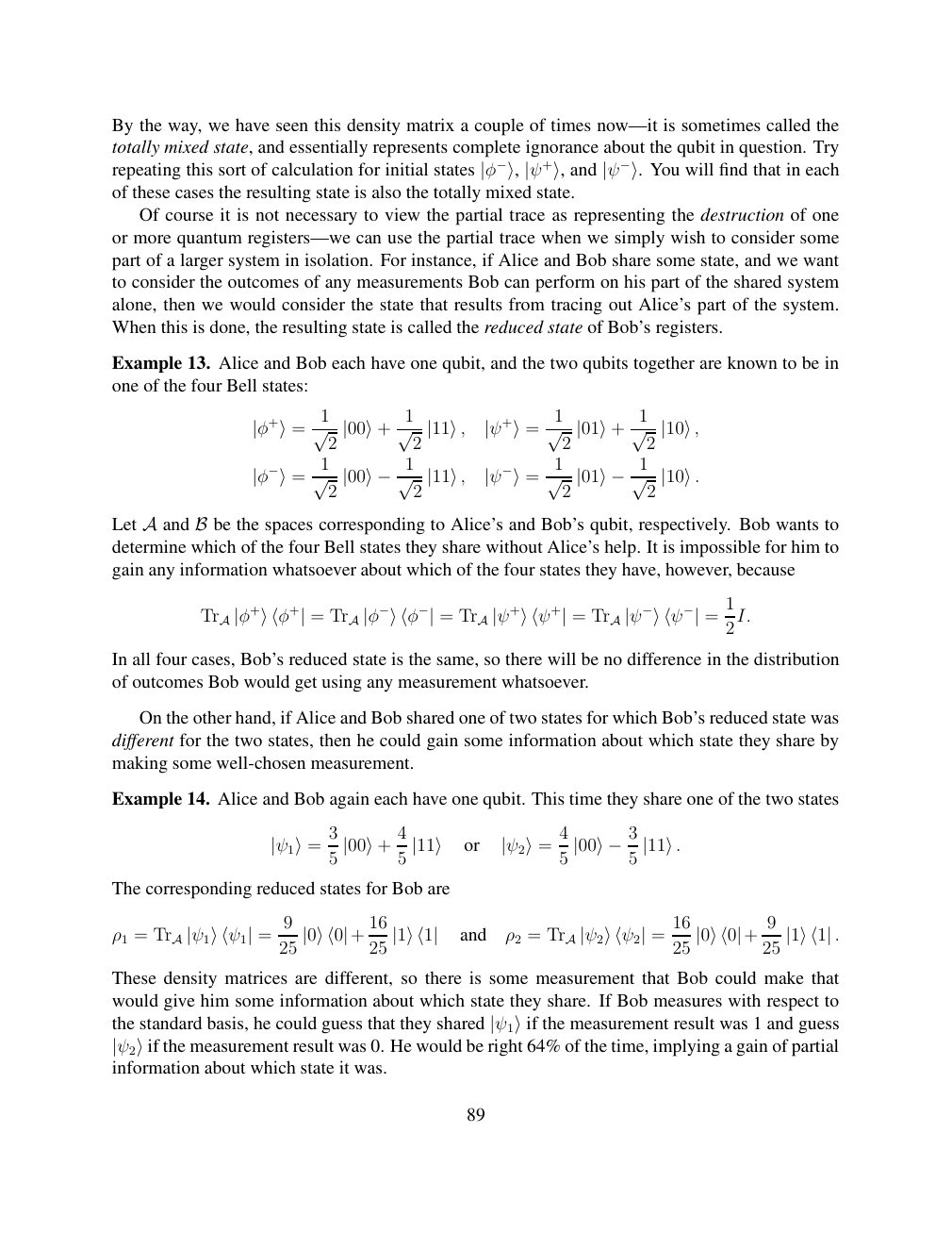
Show extracted searchable text (mathematical glyphs may differ)
By the way, we have seen this density matrix a couple of times now—it is sometimes called the
totally mixed state, and essentially represents complete ignorance about the qubit in question. Try
repeating this sort of calculation for initial states |φ−⟩, |ψ+⟩, and |ψ−⟩. You will find that in eachof these cases the resulting state is also the totally mixed state.
Of course it is not necessary to view the partial trace as representing the destruction of one
or more quantum registers—we can use the partial trace when we simply wish to consider some
part of a larger system in isolation. For instance, if Alice and Bob share some state, and we want
to consider the outcomes of any measurements Bob can perform on his part of the shared system
alone, then we would consider the state that results from tracing out Alice’s part of the system.
When this is done, the resulting state is called the reduced state of Bob’s registers.
Example 13. Alice and Bob each have one qubit, and the two qubits together are known to be in
one of the four Bell states:
1 1 1 1
|φ+⟩= √ 2 |00⟩+ √ 2 |11⟩, |ψ+⟩= √ 2 |01⟩+ √ 2 |10⟩,
1 1
|φ−⟩= √ 2 |00⟩−1√ 2 |11⟩, |ψ−⟩= √ 2 |01⟩−1√ 2 |10⟩.
Let and be the spaces corresponding to Alice’s and Bob’s qubit, respectively. Bob wants to A Bdetermine which of the four Bell states they share without Alice’s help. It is impossible for him to
gain any information whatsoever about which of the four states they have, however, because
1
TrA |φ+⟩⟨φ+| = TrA |φ−⟩⟨φ−| = TrA |ψ+⟩⟨ψ+| = TrA |ψ−⟩⟨ψ−| = 2I.
In all four cases, Bob’s reduced state is the same, so there will be no difference in the distribution
of outcomes Bob would get using any measurement whatsoever.
On the other hand, if Alice and Bob shared one of two states for which Bob’s reduced state was
different for the two states, then he could gain some information about which state they share by
making some well-chosen measurement.
Example 14. Alice and Bob again each have one qubit. This time they share one of the two states
3 4 4
or |ψ1⟩= 5 |00⟩+ 5 |11⟩ |ψ2⟩= 5 |00⟩−35 |11⟩.
The corresponding reduced states for Bob are
9 16 16 9
ρ1 = = and ρ2 = = . TrA |ψ1⟩⟨ψ1| 25 |0⟩⟨0|+ 25 |1⟩⟨1| TrA |ψ2⟩⟨ψ2| 25 |0⟩⟨0|+ 25 |1⟩⟨1|
These density matrices are different, so there is some measurement that Bob could make that
would give him some information about which state they share. If Bob measures with respect to
the standard basis, he could guess that they shared |ψ1⟩if the measurement result was 1 and guess
|ψ2⟩if the measurement result was 0. He would be right 64% of the time, implying a gain of partialinformation about which state it was.
89
Source page 90
Direct link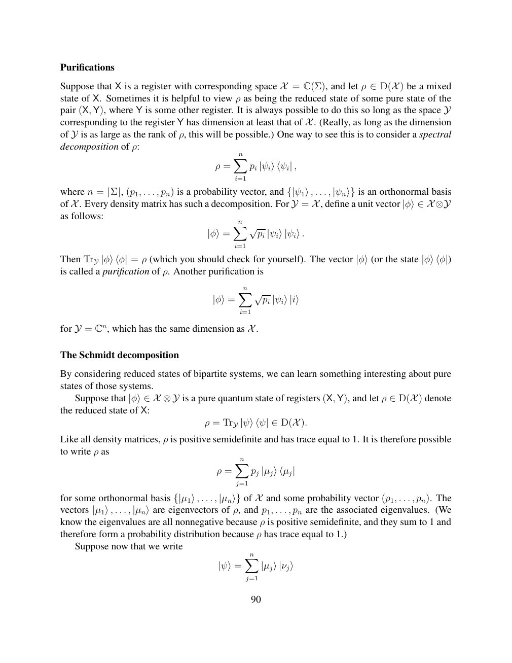
Show extracted searchable text (mathematical glyphs may differ)
Purifications
Suppose that X is a register with corresponding space = C(Σ), and let ρ ) be a mixed X ∈D(Xstate of X. Sometimes it is helpful to view ρ as being the reduced state of some pure state of the
pair (X, Y), where Y is some other register. It is always possible to do this so long as the space Y Ycorresponding to the register has dimension at least that of . (Really, as long as the dimension Xof is as large as the rank of ρ, this will be possible.) One way to see this is to consider a spectral Ydecomposition of ρ:
Xn
ρ = pi |ψi⟩⟨ψi| ,
i=1
is an orthonormal basis (p1, . . . , pn) is a probability vector, andwhere n = |Σ|, {|ψ1⟩, . . . , |ψn⟩}of . Every density matrix has such a decomposition. For = , define a unit vector X Y X |φ⟩∈X ⊗Yas follows:
Xn
√pi |φ⟩= |ψi⟩|ψi⟩.
i=1
Then = ρ (which you should check for yourself). The vector the state TrY |φ⟩⟨φ| |φ⟩(or |φ⟩⟨φ|)is called a purification of ρ. Another purification is
Xn
√pi |φ⟩= |ψi⟩|i⟩
i=1
for = Cn, which has the same dimension as . Y X
The Schmidt decomposition
By considering reduced states of bipartite systems, we can learn something interesting about pure
states of those systems.
Suppose that is a pure quantum state of registers (X, Y), and let ρ ) denote |φ⟩∈X ⊗Y ∈D(Xthe reduced state of X:
ρ = TrY |ψ⟩⟨ψ| ∈D(X ).
Like all density matrices, ρ is positive semidefinite and has trace equal to 1. It is therefore possible
to write ρ as
Xn
ρ = pj |µj⟩⟨µj|
j=1
for some orthonormal basis . . . , of and some probability vector (p1, . . . , pn). The {|µ1⟩, |µn⟩} Xvectors . . . , eigenvectors of ρ, and p1, . . . , pn are the associated eigenvalues. (We |µ1⟩, |µn⟩areknow the eigenvalues are all nonnegative because ρ is positive semidefinite, and they sum to 1 and
therefore form a probability distribution because ρ has trace equal to 1.)
Suppose now that we write
Xn
|ψ⟩= |µj⟩|νj⟩
j=1
90
Source page 91
Direct link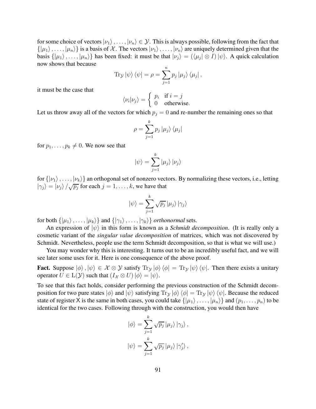
Show extracted searchable text (mathematical glyphs may differ)
for some choice of vectors . . . , This is always possible, following from the fact that |ν1⟩, |νn⟩∈Y. . . . , is a basis of . The vectors . . . , uniquely determined given that the{|µ1⟩, |µn⟩} X |ν1⟩, |νn⟩arebasis . . . , has been fixed: it must be that A quick calculation {|µ1⟩, |µn⟩} |νj⟩= (⟨µj| ⊗I) |ψ⟩.now shows that because
Xn
TrY |ψ⟩⟨ψ| = ρ = pj |µj⟩⟨µj| ,
j=1
it must be the case that
pi if i = j
⟨νi|νj⟩= 0 otherwise.
Let us throw away all of the vectors for which pj = 0 and re-number the remaining ones so that
Xk
ρ = pj |µj⟩⟨µj|
j=1
for p1, . . . , pk 0. We now see that ̸=
Xk
|ψ⟩= |µj⟩|νj⟩
j=1
for . . . , an orthogonal set of nonzero vectors. By normalizing these vectors, i.e., letting {|ν1⟩, |νk⟩} for each j = 1, . . . , k, we have that|γj⟩= |νj⟩/√pj
Xk
√pj |ψ⟩= |µj⟩|γj⟩
j=1
for both . . . , and . . . , orthonormal sets. {|µ1⟩, |µk⟩} {|γ1⟩, |γk⟩}
An expression of |ψ⟩in this form is known as a Schmidt decomposition. (It is really only acosmetic variant of the singular value decomposition of matrices, which was not discovered by
Schmidt. Nevertheless, people use the term Schmidt decomposition, so that is what we will use.)
You may wonder why this is interesting. It turns out to be an incredibly useful fact, and we will
see later some uses for it. Here is one consequence of the above proof.
Fact. Suppose satisfy = Then there exists a unitary |φ⟩, |ψ⟩∈X ⊗Y TrY |φ⟩⟨φ| TrY |ψ⟩⟨ψ|.operator U such that ∈L(Y) (IX ⊗U) |φ⟩= |ψ⟩.
To see that this fact holds, consider performing the previous construction of the Schmidt decom-
position for two pure states = Because the reduced TrY |φ⟩and |ψ⟩satisfying |φ⟩⟨φ| TrY |ψ⟩⟨ψ|. . . .state of register X is the same in both cases, you could take , and (p1, . . . , pn) to be {|µ1⟩, |µn⟩}identical for the two cases. Following through with the construction, you would then have
Xk
√pj |φ⟩= |µj⟩|γj⟩,
j=1
Xk
√pj |ψ⟩= |µj⟩|γ′j⟩,
j=1
91
Source page 92
Direct link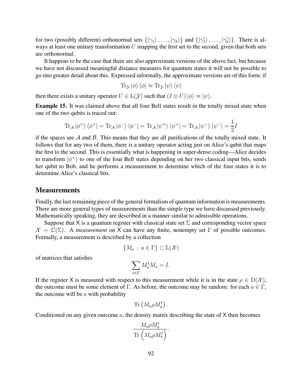
Show extracted searchable text (mathematical glyphs may differ)
for two (possibly different) orthonormal sets . . . , and . . . , There is al- {|γ1⟩, |γk⟩} {|γ′1⟩, |γ′k⟩}.ways at least one unitary transformation U mapping the first set to the second, given that both sets
are orthonormal.
It happens to be the case that there are also approximate versions of the above fact, but because
we have not discussed meaningful distance measures for quantum states it will not be possible to
go into greater detail about this. Expressed informally, the approximate versions are of this form: if
TrY |φ⟩⟨φ| ≈TrY |ψ⟩⟨ψ|
then there exists a unitary operator U such that (I ∈L(Y) ⊗U) |φ⟩≈|ψ⟩.
Example 15. It was claimed above that all four Bell states result in the totally mixed state when
one of the two qubits is traced out:
1
TrA |φ+⟩⟨φ+| = TrA |φ−⟩⟨φ−| = TrA |ψ+⟩⟨ψ+| = TrA |ψ−⟩⟨ψ−| = 2I
if the spaces are and This means that they are all purifications of the totally mixed state. It A B.follows that for any two of them, there is a unitary operator acting just on Alice’s qubit that maps
the first to the second. This is essentially what is happening in super-dense coding—Alice decides
to transform |φ+⟩to one of the four Bell states depending on her two classical input bits, sendsher qubit to Bob, and he performs a measurement to determine which of the four states it is to
determine Alice’s classical bits.
Measurements
Finally, the last remaining piece of the general formalism of quantum information is measurements.
There are more general types of measurements than the simple type we have discussed previously.
Mathematically speaking, they are described in a manner similar to admissible operations.
Suppose that X is a quantum register with classical state set Σ and corresponding vector space
= C(Σ). A measurement on X can have any finite, nonempty set Γ of possible outcomes.XFormally, a measurement is described by a collection
{Ma : a ∈Γ} ⊂L(X )
of matrices that satisfies X
M aMa† = I.
a∈Γ
If the register X is measured with respect to this measurement while it is in the state ρ ), ∈D(X
the outcome must be some element of Γ. As before, the outcome may be random: for each a ∈Γ,the outcome will be a with probability
Tr MaρM a† .
Conditioned on any given outcome a, the density matrix describing the state of X then becomes
MaρM a†
.
Tr MaρM a†
92
Source page 93
Direct link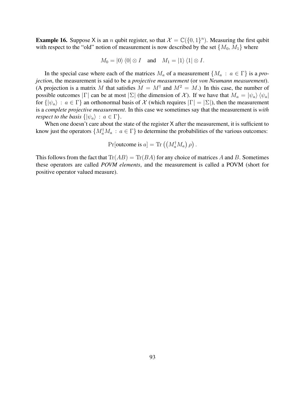
Show extracted searchable text (mathematical glyphs may differ)
Example 16. Suppose X is an n qubit register, so that = Measuring the first qubit X C({0, 1}n).with respect to the “old” notion of measurement is now described by the set where {M0, M1}
M0 = and M1 = |0⟩⟨0| ⊗I |1⟩⟨1| ⊗I.
In the special case where each of the matrices Ma of a measurement : a is a pro- {Ma ∈Γ}jection, the measurement is said to be a projective measurement (or von Neumann measurement).
(A projection is a matrix M that satisfies M = M † and M 2 = M.) In this case, the number of
possible outcomes can be at most (the dimension of ). If we have that Ma = |Γ| |Σ| X |ψa⟩⟨ψa|for a an orthonormal basis of (which requires = then the measurement {|ψa⟩: ∈Γ} X |Γ| |Σ|),is a complete projective measurement. In this case we sometimes say that the measurement is with
respect to the basis {|ψa⟩: a ∈Γ}. When one doesn’t care about the state of the register X after the measurement, it is sufficient to
know just the operators aMa† : a to determine the probabilities of the various outcomes: {M ∈Γ}
Pr[outcome is a] = Tr M aMa† ρ .
This follows from the fact that Tr(AB) = Tr(BA) for any choice of matrices A and B. Sometimes
these operators are called POVM elements, and the measurement is called a POVM (short for
positive operator valued measure).
93
⊗ Circuit walkthrough: entanglement and measurement
The Hadamard gate prepares (|0⟩ + |1⟩)/√2 on the first qubit. The controlled-NOT then creates the Bell state (|00⟩ + |11⟩)/√2. Measuring both qubits in the computational basis produces correlated 00 and 11 outcomes, each with ideal probability 1/2. This example illustrates a circuit building block; it is not a complete implementation of the surrounding algorithm.
Show runnable Qiskit example
from qiskit import QuantumCircuit
from qiskit_aer import AerSimulator

qc = QuantumCircuit(2, 2)
qc.h(0)             # Superpose the first qubit
qc.cx(0, 1)         # Entangle both qubits
qc.measure([0, 1], [0, 1])
print(qc.draw(output="text"))
result = AerSimulator().run(qc, shots=1024).result()
print(result.get_counts())  # Approximately 00 and 11
Install qiskit and qiskit-aer locally to execute this code. The diagram is a static circuit illustration, not a browser-based simulator.