Math fidelity: The original PDF page is displayed as a high-resolution image so that equations, bra–ket notation, matrix layouts and circuit diagrams remain exactly as in the source. The expandable text layer is for searching and may not reproduce every mathematical glyph.
Source page 120
Direct link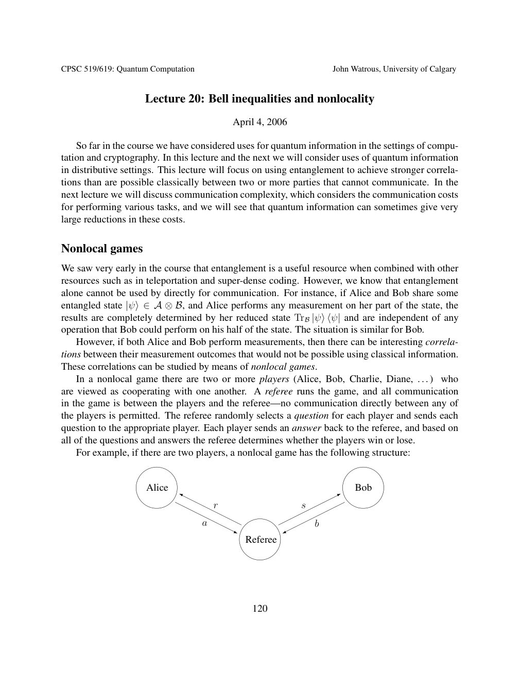
Show extracted searchable text (mathematical glyphs may differ)
CPSC 519/619: Quantum Computation John Watrous, University of Calgary
Lecture 20: Bell inequalities and nonlocality
April 4, 2006
So far in the course we have considered uses for quantum information in the settings of compu-
tation and cryptography. In this lecture and the next we will consider uses of quantum information
in distributive settings. This lecture will focus on using entanglement to achieve stronger correla-
tions than are possible classically between two or more parties that cannot communicate. In the
next lecture we will discuss communication complexity, which considers the communication costs
for performing various tasks, and we will see that quantum information can sometimes give very
large reductions in these costs.
Nonlocal games
We saw very early in the course that entanglement is a useful resource when combined with other
resources such as in teleportation and super-dense coding. However, we know that entanglement
alone cannot be used by directly for communication. For instance, if Alice and Bob share some
entangled state and Alice performs any measurement on her part of the state, the |ψ⟩∈A ⊗B,results are completely determined by her reduced state and are independent of any TrB |ψ⟩⟨ψ|operation that Bob could perform on his half of the state. The situation is similar for Bob.
However, if both Alice and Bob perform measurements, then there can be interesting correla-
tions between their measurement outcomes that would not be possible using classical information.
These correlations can be studied by means of nonlocal games.
In a nonlocal game there are two or more players (Alice, Bob, Charlie, Diane, . . . ) who
are viewed as cooperating with one another. A referee runs the game, and all communication
in the game is between the players and the referee—no communication directly between any of
the players is permitted. The referee randomly selects a question for each player and sends each
question to the appropriate player. Each player sends an answer back to the referee, and based on
all of the questions and answers the referee determines whether the players win or lose.
For example, if there are two players, a nonlocal game has the following structure:
Alice Bob
Y *
r s
a b j
Referee
120
Source page 121
Direct link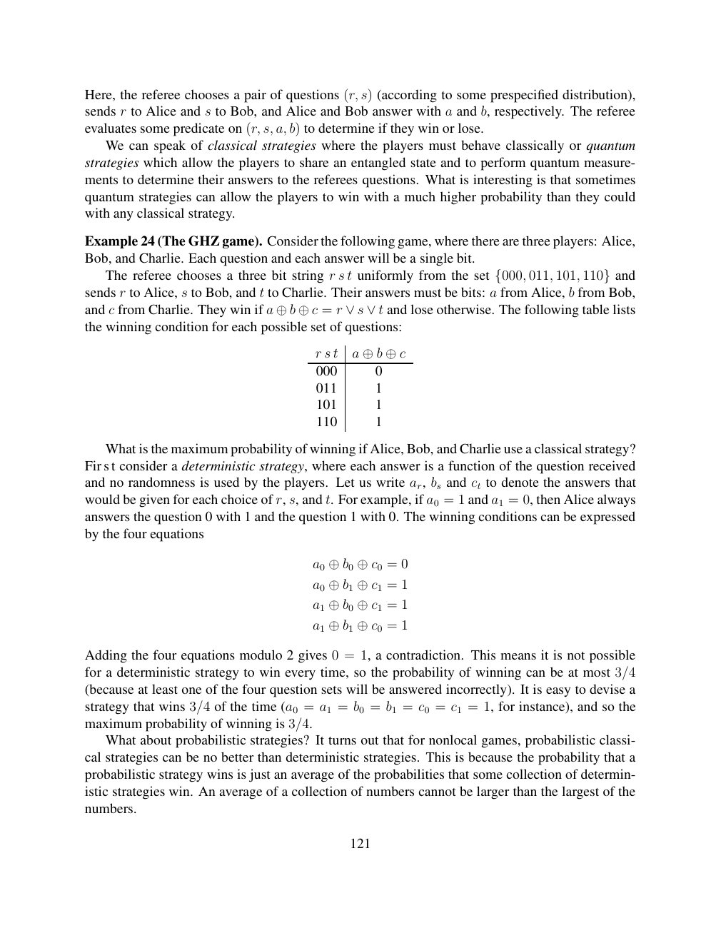
Show extracted searchable text (mathematical glyphs may differ)
Here, the referee chooses a pair of questions (r, s) (according to some prespecified distribution),
sends r to Alice and s to Bob, and Alice and Bob answer with a and b, respectively. The referee
evaluates some predicate on (r, s, a, b) to determine if they win or lose.
We can speak of classical strategies where the players must behave classically or quantum
strategies which allow the players to share an entangled state and to perform quantum measure-
ments to determine their answers to the referees questions. What is interesting is that sometimes
quantum strategies can allow the players to win with a much higher probability than they could
with any classical strategy.
Example 24 (The GHZ game). Consider the following game, where there are three players: Alice,
Bob, and Charlie. Each question and each answer will be a single bit.
The referee chooses a three bit string r s t uniformly from the set 011, 101, and {000, 110}sends r to Alice, s to Bob, and t to Charlie. Their answers must be bits: a from Alice, b from Bob,
and c from Charlie. They win if a = r and lose otherwise. The following table lists ⊕b ⊕c ∨s ∨tthe winning condition for each possible set of questions:
r s t a ⊕b ⊕c 000 0
011 1
101 1
110 1
What is the maximum probability of winning if Alice, Bob, and Charlie use a classical strategy?
Fir s t consider a deterministic strategy, where each answer is a function of the question received
and no randomness is used by the players. Let us write ar, bs and ct to denote the answers that
would be given for each choice of r, s, and t. For example, if a0 = 1 and a1 = 0, then Alice always
answers the question 0 with 1 and the question 1 with 0. The winning conditions can be expressed
by the four equations
a0 ⊕b0 ⊕c0 = 0
a0 ⊕b1 ⊕c1 = 1
a1 ⊕b0 ⊕c1 = 1
a1 ⊕b1 ⊕c0 = 1
Adding the four equations modulo 2 gives 0 = 1, a contradiction. This means it is not possible
for a deterministic strategy to win every time, so the probability of winning can be at most 3/4
(because at least one of the four question sets will be answered incorrectly). It is easy to devise a
strategy that wins 3/4 of the time (a0 = a1 = b0 = b1 = c0 = c1 = 1, for instance), and so the
maximum probability of winning is 3/4.
What about probabilistic strategies? It turns out that for nonlocal games, probabilistic classi-
cal strategies can be no better than deterministic strategies. This is because the probability that a
probabilistic strategy wins is just an average of the probabilities that some collection of determin-
istic strategies win. An average of a collection of numbers cannot be larger than the largest of the
numbers.
121
Source page 122
Direct link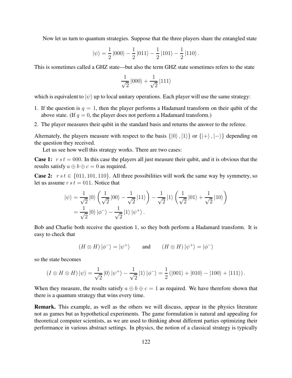
Show extracted searchable text (mathematical glyphs may differ)
Now let us turn to quantum strategies. Suppose that the three players share the entangled state
1
|ψ⟩= 2 |000⟩−12 |011⟩−12 |101⟩−12 |110⟩.
This is sometimes called a GHZ state—but also the term GHZ state sometimes refers to the state
1 1
√ 2 |000⟩+ √ 2 |111⟩
which is equivalent to |ψ⟩up to local unitary operations. Each player will use the same strategy:
1. If the question is q = 1, then the player performs a Hadamard transform on their qubit of the
above state. (If q = 0, the player does not perform a Hadamard transform.)
2. The player measures their qubit in the standard basis and returns the answer to the referee.
Alternately, the players measure with respect to the basis or depending on {|0⟩, |1⟩} {|+⟩, |−⟩}the question they received.
Let us see how well this strategy works. There are two cases:
Case 1: r s t = 000. In this case the players all just measure their qubit, and it is obvious that the
results satisfy a = 0 as required. ⊕b ⊕c
Case 2: r s t 101, All three possibilities will work the same way by symmetry, so ∈{011, 110}.let us assume r s t = 011. Notice that
1 1 1 1
|ψ⟩= √ 2 |0⟩ √ 2 |00⟩−1√ 2 |11⟩ −1√ 2 |1⟩ √ 2 |01⟩+ √ 2 |10⟩
1
= √ 2 |0⟩|φ−⟩−1√ 2 |1⟩|ψ+⟩.
Bob and Charlie both receive the question 1, so they both perform a Hadamard transform. It is
easy to check that
(H and (H ⊗H) |φ−⟩= |ψ+⟩ ⊗H) |ψ+⟩= |φ−⟩
so the state becomes
1 1
. (I ⊗H ⊗H) |ψ⟩= √ 2 |0⟩|ψ+⟩−1√ 2 |1⟩|φ−⟩= 2 (|001⟩+ |010⟩−|100⟩+ |111⟩)
When they measure, the results satisfy a = 1 as required. We have therefore shown that ⊕b ⊕cthere is a quantum strategy that wins every time.
Remark. This example, as well as the others we will discuss, appear in the physics literature
not as games but as hypothetical experiments. The game formulation is natural and appealing for
theoretical computer scientists, as we are used to thinking about different parties optimizing their
performance in various abstract settings. In physics, the notion of a classical strategy is typically
122
Source page 123
Direct link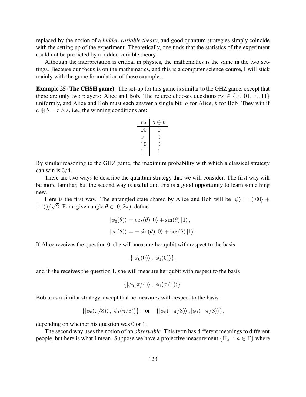
Show extracted searchable text (mathematical glyphs may differ)
replaced by the notion of a hidden variable theory, and good quantum strategies simply coincide
with the setting up of the experiment. Theoretically, one finds that the statistics of the experiment
could not be predicted by a hidden variable theory.
Although the interpretation is critical in physics, the mathematics is the same in the two set-
tings. Because our focus is on the mathematics, and this is a computer science course, I will stick
mainly with the game formulation of these examples.
Example 25 (The CHSH game). The set-up for this game is similar to the GHZ game, except that
there are only two players: Alice and Bob. The referee chooses questions rs 01, 10, ∈{00, 11}uniformly, and Alice and Bob must each answer a single bit: a for Alice, b for Bob. They win if
a = r i.e., the winning conditions are: ⊕b ∧s,
rs a ⊕b 00 0
01 0
10 0
11 1
By similar reasoning to the GHZ game, the maximum probability with which a classical strategy
can win is 3/4.
There are two ways to describe the quantum strategy that we will consider. The first way will
be more familiar, but the second way is useful and this is a good opportunity to learn something
new.
Here is the first way. The entangled state shared by Alice and Bob will be |ψ⟩= (|00⟩+ √ 2. For a given angle θ 2π), define|11⟩)/ ∈[0,
|φ0(θ)⟩= cos(θ) |0⟩+ sin(θ) |1⟩,
|φ1(θ)⟩= −sin(θ) |0⟩+ cos(θ) |1⟩.
If Alice receives the question 0, she will measure her qubit with respect to the basis
{|φ0(0)⟩, |φ1(0)⟩},
and if she receives the question 1, she will measure her qubit with respect to the basis
{|φ0(π/4)⟩, |φ1(π/4)⟩}.
Bob uses a similar strategy, except that he measures with respect to the basis
or {|φ0(π/8)⟩, |φ1(π/8)⟩} {|φ0(−π/8)⟩, |φ1(−π/8)⟩},
depending on whether his question was 0 or 1.
The second way uses the notion of an observable. This term has different meanings to different
people, but here is what I mean. Suppose we have a projective measurement : a where {Πa ∈Γ}
123
Source page 124
Direct link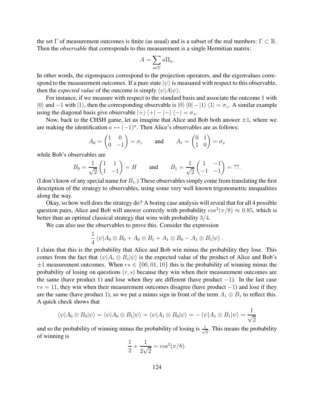
Show extracted searchable text (mathematical glyphs may differ)
the set Γ of measurement outcomes is finite (as usual) and is a subset of the real numbers: Γ ⊂R.Then the observable that corresponds to this measurement is a single Hermitian matrix:
X
A = aΠa.
a∈Γ
In other words, the eigenspaces correspond to the projection operators, and the eigenvalues corre-
spond to the measurement outcomes. If a pure state |ψ⟩is measured with respect to this observable,
then the expected value of the outcome is simply ⟨ψ|A|ψ⟩. For instance, if we measure with respect to the standard basis and associate the outcome 1 with
= σz. A similar example|0⟩and −1 with |1⟩, then the corresponding observable is |0⟩⟨0|−|1⟩⟨1|using the diagonal basis give observable = σx. |+⟩⟨+| −|−⟩⟨−|
Now, back to the CHSH game, let us imagine that Alice and Bob both answer ±1, where we
are making the identification a ↔(−1)a. Then Alice’s observables are as follows:
1 0 0 1 A0 = = σz and A1 = = σx
0 −1 1 0
while Bob’s observables are
1 1 1 1 1 B0 = = H and B1 = −1 = ??. √ 2 1 √ 2 −1 −1 −1
(I don’t know of any special name for B1.) These observables simply come from translating the first
description of the strategy to observables, using some very well known trigonometric inequalities
along the way.
Okay, so how well does the strategy do? A boring case analysis will reveal that for all 4 possible
question pairs, Alice and Bob will answer correctly with probability cos2(π/8) ≈0.85, which isbetter than an optimal classical strategy that wins with probability 3/4.
We can also use the observables to prove this. Consider the expression
1
+ A0 + A1 4 ⟨ψ|A0 ⊗B0 ⊗B1 ⊗B0 −A1 ⊗B1|ψ⟩.
I claim that this is the probability that Alice and Bob win minus the probability they lose. This
comes from the fact that the expected value of the product of Alice and Bob’s ⟨ψ|Ar ⊗Bs|ψ⟩is measurement outcomes. When rs 01, this is the probability of winning minus the±1 ∈{00, 10}probability of losing on questions (r, s) because they win when their measurement outcomes are
the same (have product 1) and lose when they are different (have product −1). In the last case
rs = 11, they win when their measurement outcomes disagree (have product −1) and lose if theyare the same (have product 1), so we put a minus sign in front of the term A1 to reflect this. ⊗B1A quick check shows that
1
⟨ψ|A0 ⊗B0|ψ⟩= ⟨ψ|A0 ⊗B1|ψ⟩= ⟨ψ|A1 ⊗B0|ψ⟩= −⟨ψ|A1 ⊗B1|ψ⟩= √ 2
and so the probability of winning minus the probability of losing is √12. This means the probability
of winning is
1 1
+
2 2 √ 2 = cos2(π/8).
124
Source page 125
Direct link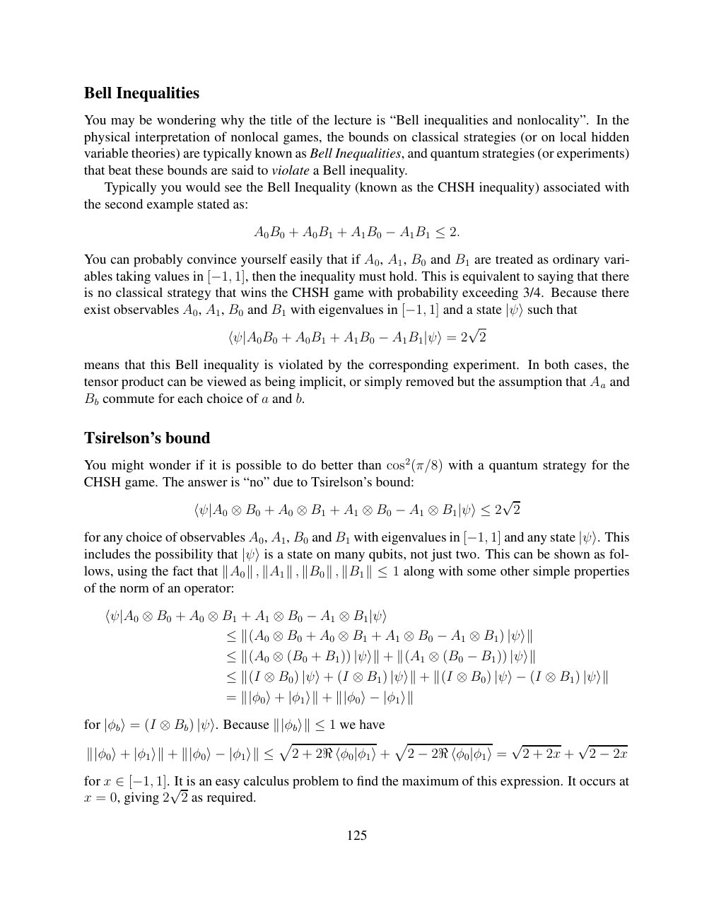
Show extracted searchable text (mathematical glyphs may differ)
Bell Inequalities
You may be wondering why the title of the lecture is “Bell inequalities and nonlocality”. In the
physical interpretation of nonlocal games, the bounds on classical strategies (or on local hidden
variable theories) are typically known as Bell Inequalities, and quantum strategies (or experiments)
that beat these bounds are said to violate a Bell inequality.
Typically you would see the Bell Inequality (known as the CHSH inequality) associated with
the second example stated as:
A0B0 + A0B1 + A1B0 −A1B1 ≤2.
You can probably convince yourself easily that if A0, A1, B0 and B1 are treated as ordinary vari-
ables taking values in 1], then the inequality must hold. This is equivalent to saying that there [−1,is no classical strategy that wins the CHSH game with probability exceeding 3/4. Because there
exist observables A0, A1, B0 and B1 with eigenvalues in 1] and a state that [−1, |ψ⟩such
+ A0B1 + A1B0 2 √2 ⟨ψ|A0B0 −A1B1|ψ⟩=
means that this Bell inequality is violated by the corresponding experiment. In both cases, the
tensor product can be viewed as being implicit, or simply removed but the assumption that Aa and
Bb commute for each choice of a and b.
Tsirelson’s bound
You might wonder if it is possible to do better than cos2(π/8) with a quantum strategy for the
CHSH game. The answer is “no” due to Tsirelson’s bound:
+ A0 + A1 √2 ⟨ψ|A0 ⊗B0 ⊗B1 ⊗B0 −A1 ⊗B1|ψ⟩≤2
for any choice of observables A0, A1, B0 and B1 with eigenvalues in 1] and any state This [−1, |ψ⟩.
includes the possibility that |ψ⟩is a state on many qubits, not just two. This can be shown as fol-lows, using the fact that along with some other simple properties ∥A0∥, ∥A1∥, ∥B0∥, ∥B1∥≤1of the norm of an operator:
⟨ψ|A0 ⊗B0 + A0 ⊗B1 + A1 ⊗B0 −A1 ⊗B1|ψ⟩
≤∥(A0 ⊗B0 + A0 ⊗B1 + A1 ⊗B0 −A1 ⊗B1) |ψ⟩∥
≤∥(A0 ⊗(B0 + B1)) |ψ⟩∥+ ∥(A1 ⊗(B0 −B1)) |ψ⟩∥
≤∥(I ⊗B0) |ψ⟩+ (I ⊗B1) |ψ⟩∥+ ∥(I ⊗B0) |ψ⟩−(I ⊗B1) |ψ⟩∥
= ∥|φ0⟩+ |φ1⟩∥+ ∥|φ0⟩−|φ1⟩∥
for (I Because we have |φb⟩= ⊗Bb) |ψ⟩. ∥|φb⟩∥≤1 p p
2 + 2 √ 2 + 2x + √2∥|φ0⟩+ |φ1⟩∥+ ∥|φ0⟩−|φ1⟩∥≤ 2ℜ⟨φ0|φ1⟩+ −2ℜ⟨φ0|φ1⟩= −2x
for x 1]. It is an easy calculus problem to find the maximum of this expression. It occurs at ∈[−1,x = 0, giving 2 √ 2 as required.
125
⊗ Circuit walkthrough: entanglement and measurement
The Hadamard gate prepares (|0⟩ + |1⟩)/√2 on the first qubit. The controlled-NOT then creates the Bell state (|00⟩ + |11⟩)/√2. Measuring both qubits in the computational basis produces correlated 00 and 11 outcomes, each with ideal probability 1/2. This example illustrates a circuit building block; it is not a complete implementation of the surrounding algorithm.
Show runnable Qiskit example
from qiskit import QuantumCircuit
from qiskit_aer import AerSimulator

qc = QuantumCircuit(2, 2)
qc.h(0)             # Superpose the first qubit
qc.cx(0, 1)         # Entangle both qubits
qc.measure([0, 1], [0, 1])
print(qc.draw(output="text"))
result = AerSimulator().run(qc, shots=1024).result()
print(result.get_counts())  # Approximately 00 and 11
Install qiskit and qiskit-aer locally to execute this code. The diagram is a static circuit illustration, not a browser-based simulator.